Hardy-Weinberg for IB Biology (HL Guide)

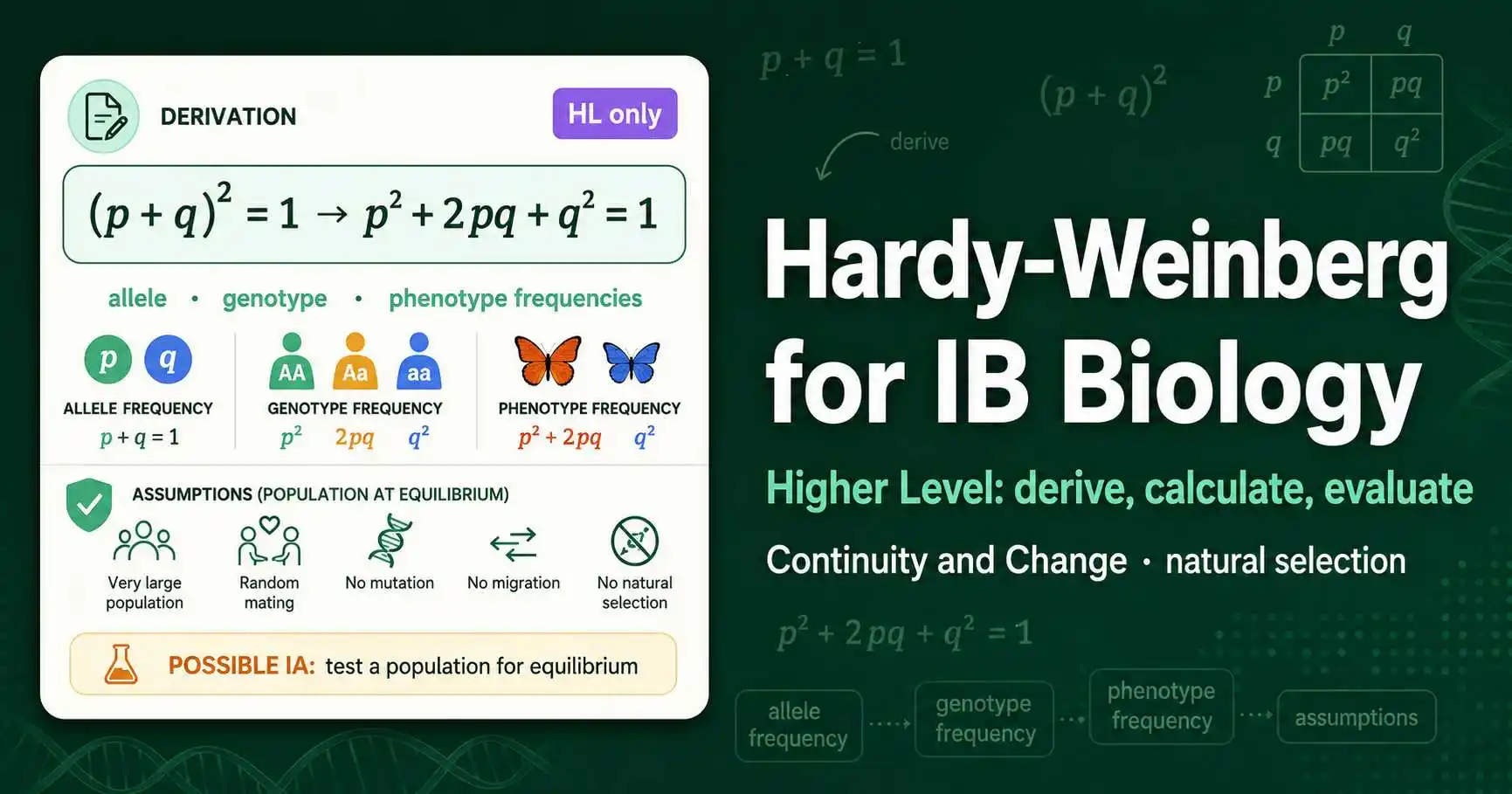
In IB Biology, Hardy-Weinberg is a Higher Level topic, found in the additional higher level material on natural selection within the Continuity and Change theme. Unlike some courses, IB asks you not just to use the equation but to derive it, to calculate allele, genotype, and phenotype frequencies, and to state the assumptions behind it. The two equations are p + q = 1 for alleles and p² + 2pq + q² = 1 for genotypes, and HL students need to understand where the second comes from, not merely how to apply it.

This guide covers Hardy-Weinberg specifically for the IB Biology HL course, aligned with the current syllabus: why it is HL-only, how to derive the equation as the syllabus requires, the full calculation method including phenotype frequencies, the assumptions you must be able to state, and how the topic appears in exams and potentially the internal assessment. The IB approach rewards genuine understanding over memorization, which suits this topic well. The calculations can be practised with a calculator while building the conceptual grasp the IB expects.

Where Hardy-Weinberg Sits in IB Biology

Hardy-Weinberg is part of the additional higher level content in IB Biology, which means it is studied by HL students but not by Standard Level students. It falls under the natural selection material in the Continuity and Change theme, connecting the genetics of inheritance to the evolution of populations.

This HL-only placement matters for how you should approach the topic. Because it is higher level material, the IB expects a deeper treatment than a surface formula. HL students are asked to understand the principle conceptually, derive its central equation, apply it to calculations, and articulate the conditions under which it holds. Standard Level students do not need this material, so if you are studying SL, Hardy-Weinberg is outside your syllabus, while HL students should treat it as examinable content that can appear in calculations and explanations.

The placement within natural selection also frames the biological meaning. The IB presents Hardy-Weinberg as describing a population in which allele frequencies remain constant, that is, a population not currently undergoing evolution. This connects directly to the surrounding HL content on evolution, gene pools, and speciation, where changes in allele frequencies are the substance of evolutionary change. Understanding Hardy-Weinberg as the no-change baseline helps you see why deviations from it are evidence of the evolutionary processes the rest of the theme explores. The principle describes a population whose allele and genotype frequencies stay constant from generation to generation when no evolutionary force acts on it.

Deriving the Equation: An IB Requirement

A distinctive feature of the IB treatment is that HL students are expected to understand how the Hardy-Weinberg equation is derived, not just to use it. This sets IB apart from courses that simply provide the equation, and it genuinely rewards students who grasp the underlying logic.

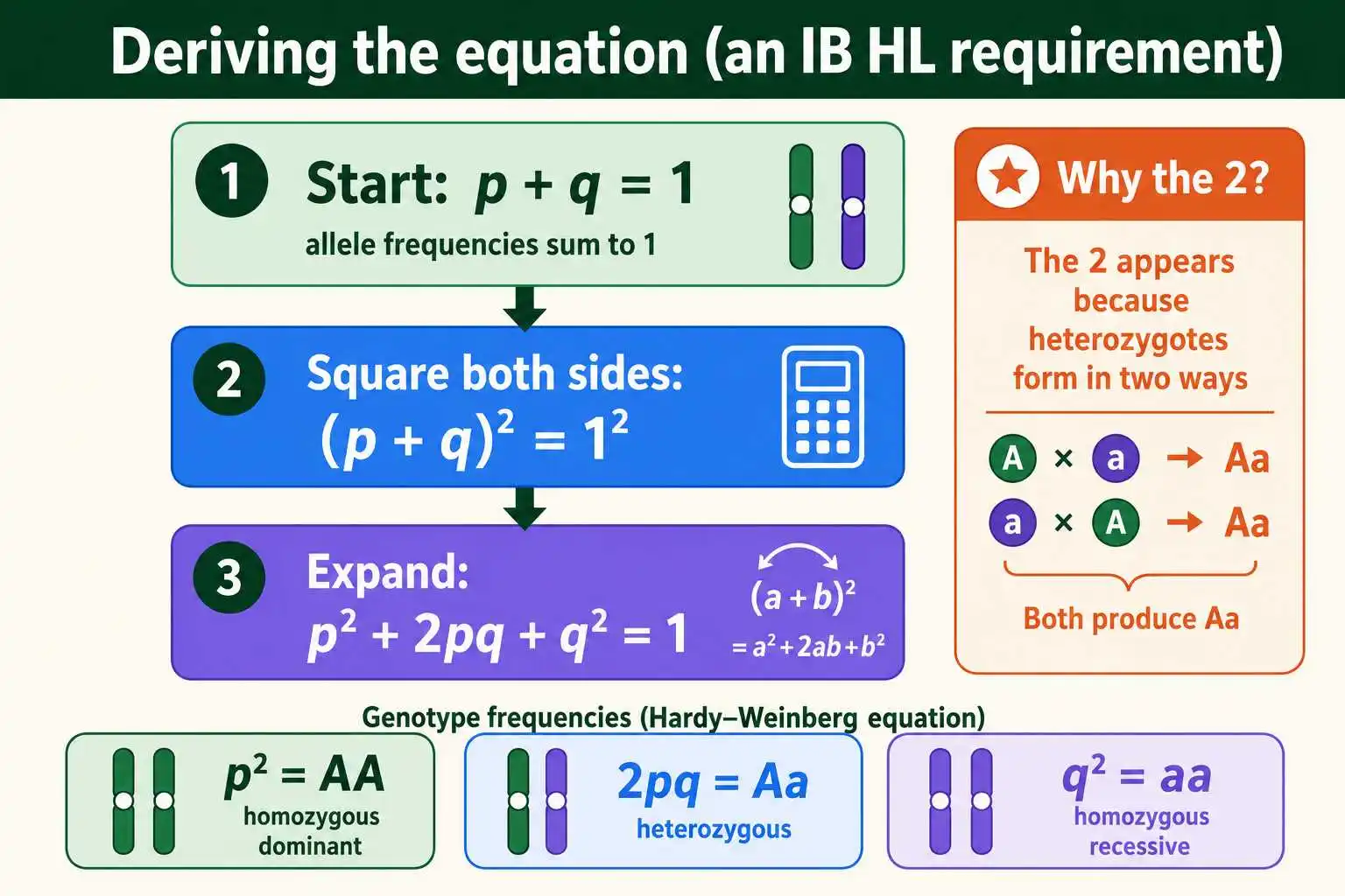
The derivation starts from the allele frequencies. For a gene with two alleles, let p be the frequency of one allele and q be the frequency of the other. Since these are the only two alleles, they account for every copy of the gene, so their frequencies sum to 1: p + q = 1. This is the first equation, and it is almost self-evident, simply stating that the two allele frequencies make up the whole.

The second equation follows by considering how alleles combine to form genotypes. When two alleles come together to form a diploid individual, the genotype frequencies are described by squaring the allele equation. Because p + q = 1, it follows that (p + q)² = 1² = 1. Expanding the left side gives p² + 2pq + q², so p² + 2pq + q² = 1. Each term corresponds to a genotype: p² is the frequency of the homozygous dominant genotype, 2pq is the frequency of the heterozygous genotype, and q² is the frequency of the homozygous recessive genotype. The 2 in the middle term arises because heterozygotes can form in two ways, receiving the dominant allele from either parent. Being able to show this derivation, from p + q = 1 to its squared expansion, is exactly what the IB syllabus asks of HL students.

Calculating Allele, Genotype, and Phenotype Frequencies

The IB syllabus explicitly requires HL students to calculate allele, genotype, and phenotype frequencies using the Hardy-Weinberg equation. This is broader than some courses, which focus only on allele and genotype frequencies, so the phenotype dimension is worth particular attention.

The standard calculation begins with the observable recessive phenotype. Take a classic IB-style example: in a population of 500 individuals, 9 percent show albinism, a recessive condition. The albino individuals are homozygous recessive, so q² equals 0.09. Take the square root to find q, which is 0.3, the recessive allele frequency. Then p equals 1 minus 0.3, which is 0.7, the dominant allele frequency. You now have the allele frequencies. For genotype frequencies, p² is 0.49 (homozygous dominant), 2pq is 2 times 0.7 times 0.3, which is 0.42 (heterozygous), and q² is 0.09 (homozygous recessive).

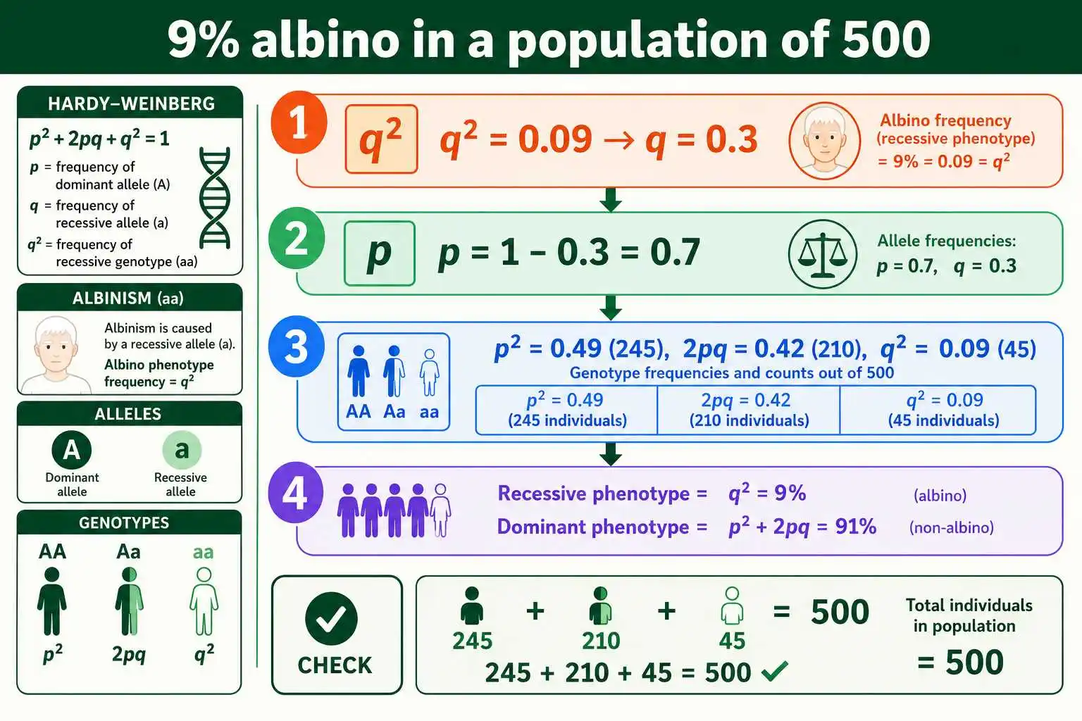
The phenotype frequencies follow from the genotypes. Because albinism is recessive, the recessive phenotype frequency is just q², which is 0.09, or 9 percent, matching the affected individuals. The dominant phenotype includes both the homozygous dominant and heterozygous individuals, since both show the normal pigmentation, so the dominant phenotype frequency is p² plus 2pq, which is 0.49 plus 0.42, equaling 0.91, or 91 percent. To convert any of these frequencies to actual numbers of individuals, multiply by the population size of 500. So the number of carriers, the heterozygotes, is 0.42 times 500, which is 210 individuals. The full mechanics of these calculations are detailed in our guide on using the Hardy-Weinberg equation.

A useful check on this albinism example shows how the numbers hang together. The three genotype frequencies, 0.49, 0.42, and 0.09, sum to 1.00 exactly, confirming the arithmetic. In terms of actual individuals out of 500, that is 245 homozygous dominant, 210 heterozygous carriers, and 45 homozygous recessive albino individuals, which add to the full 500. Notice that the 45 albino individuals are 9 percent of 500, matching the starting data, a satisfying confirmation that the whole calculation is internally consistent. This habit of converting back to counts and checking they sum to the population total is a good discipline for IB data-response questions, where a careless arithmetic slip can cost an otherwise earned mark.

The Assumptions You Must State

The IB syllabus requires HL students to state the assumptions made when the Hardy-Weinberg equation is used. These assumptions describe the conditions under which allele and genotype frequencies remain constant, and being able to list and explain them is examinable.

The assumptions are that the population is large, that mating is random, and that there is no mutation, no migration, and no natural selection. A large population avoids the random fluctuations of genetic drift. Random mating ensures alleles combine purely by chance, producing the predicted genotype proportions. No mutation means no new alleles are introduced into the gene pool. No migration means no alleles enter or leave through the movement of individuals. And no natural selection means all genotypes survive and reproduce equally, so no allele is favored over another.

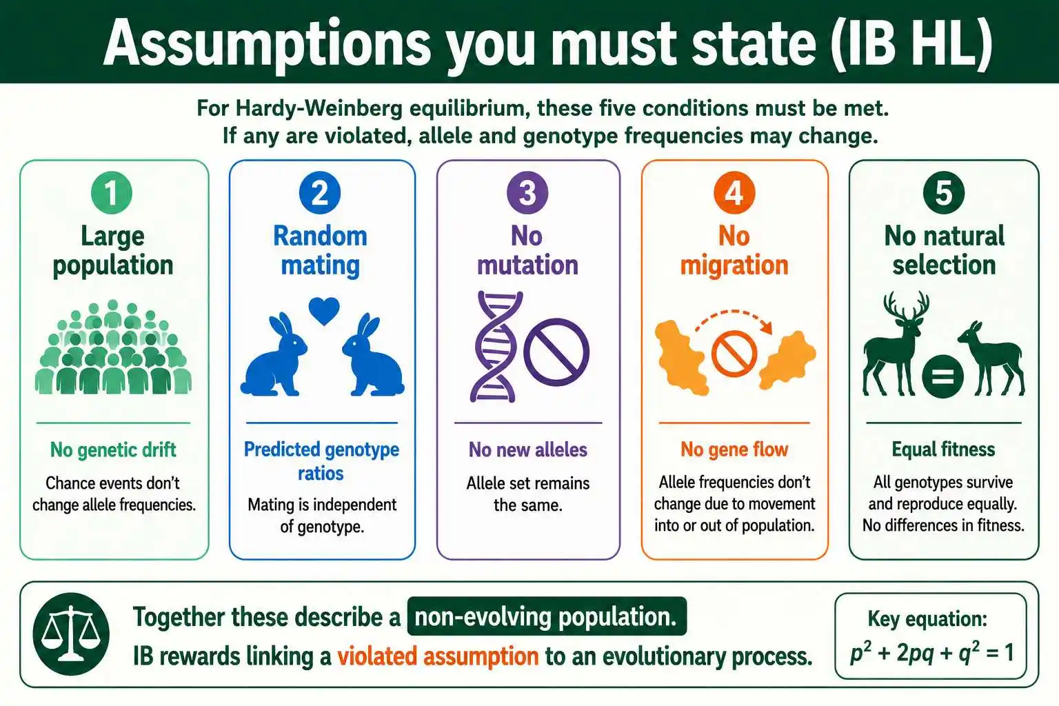
The deeper point the IB wants you to grasp is that these assumptions define a non-evolving population, and that real populations rarely meet them all. This is precisely why the equation is useful: by assuming equilibrium, you can predict expected frequencies, and any departure of real data from these predictions indicates that one of the assumptions is violated and that evolution may be occurring. When an exam question asks you to state the assumptions, listing all five clearly earns the marks, and being able to connect a violated assumption to an evolutionary mechanism demonstrates the deeper understanding HL rewards. The full treatment of each condition appears in our guide to the assumptions of Hardy-Weinberg.

How It Appears in IB Exams

In IB Biology exams, Hardy-Weinberg can appear in several forms, and knowing what to expect helps you prepare efficiently. The questions test both the calculation skills and the conceptual understanding the syllabus emphasizes.

Calculation questions provide data, typically the frequency of a recessive phenotype, and ask you to find allele, genotype, or phenotype frequencies. These follow the standard sequence: start with q², take the square root for q, find p, then compute whatever the question asks. Because IB values clear working, show each step, since method marks are often available even on data-response questions. Watch the common trap of treating the recessive phenotype frequency as q rather than q²; the square-root step is essential. Some questions may ask for the number of individuals rather than a frequency, which simply means multiplying the frequency by the population size at the end.

The mark allocation rewards a disciplined layout. On a multi-step calculation, write q² and what it represents, then the square root to q, then p from p + q = 1, then the target value, so an examiner can follow and credit each stage. Even a final answer that is slightly off from a rounding choice can still earn most of the marks if the method is shown clearly, which is why fully worked, labeled answers are always worth the few extra seconds they take.

Conceptual and explanation questions test your understanding of the principle itself. You might be asked to state the assumptions, to explain why a population is or is not in equilibrium, or to derive or justify the equation. The derivation requirement is somewhat distinctive to IB, so be ready to show how p + q = 1 leads to p² + 2pq + q² = 1 through squaring. These questions reward the conceptual depth IB cultivates, and they often connect Hardy-Weinberg to the surrounding evolution content, asking you to interpret a result in terms of evolutionary processes. This integrated reasoning mirrors how IB tests inheritance more broadly, including with the chi-square test, an approach also seen in our guide for IB Biology Punnett squares.

Connecting to the Internal Assessment

The IB internal assessment, the individual investigation, offers a possible avenue for applying Hardy-Weinberg, and understanding this connection can spark ideas for HL students designing their own investigations. While not every student will use it, the principle suits certain investigative questions well.

Hardy-Weinberg lends itself to investigations using existing datasets, often called database or secondary-data investigations, which are fully acceptable for the IA. A student might obtain published allele or genotype frequency data for a human population or another species and analyze whether the population appears to be in Hardy-Weinberg equilibrium for a particular gene. This involves calculating expected genotype frequencies from the allele frequencies and comparing them to the observed frequencies, the same logic used in statistical testing for equilibrium. Such an investigation demonstrates the data analysis and evaluation skills the IA assesses.

The key to using Hardy-Weinberg well in an IA is framing a focused research question and engaging critically with the assumptions. A strong investigation does not just compute frequencies; it discusses whether the equilibrium assumptions are reasonable for the population studied and interprets any deviation in light of possible evolutionary forces. This kind of critical evaluation, rather than mere calculation, is what earns high IA marks. Students considering this route should ensure they can access reliable genotype data and should treat the assumptions as a central part of the analysis rather than an afterthought. The statistical comparison of observed and expected frequencies connects to the method in our guide on testing Hardy-Weinberg with chi-square.

To make this concrete, a workable IA might take published genotype counts for a well-studied human polymorphism, such as the MN blood group, in one or more populations, then calculate the allele frequencies, derive the expected genotype frequencies under equilibrium, and use a chi-square test to assess whether the observed counts deviate significantly. The evaluation would then discuss which assumptions might not hold for the chosen population, perhaps non-random mating or historical migration, and what the result implies. Because the data already exist, the investigation rests on the quality of the analysis and the depth of evaluation rather than on laboratory technique, which suits students whose strengths lie in handling and interpreting data. Framing a precise research question, such as whether a named population is in equilibrium for a specific gene, keeps the investigation focused and assessable.

Common Mistakes IB Students Make

A handful of errors recur in IB Hardy-Weinberg answers, and being aware of them protects marks that are otherwise easy to earn. Most stem from rushing the method or misremembering what each symbol represents.

The most frequent error is treating the recessive phenotype frequency as q instead of q². Because the recessive phenotype corresponds to the homozygous recessive genotype, its frequency is q², so you must take the square root before using the value as an allele frequency. Skipping this step throws off every subsequent calculation. A related mistake is confusing allele frequencies with genotype frequencies, for example reporting q² when the question asked for q, or vice versa. Keeping clear which equation you are working in, p + q = 1 for alleles and p² + 2pq + q² = 1 for genotypes, prevents this.

Two further errors are specific to the IB's broader requirements. First, students sometimes forget that the dominant phenotype frequency is p² plus 2pq, not p² alone, because both homozygous dominant and heterozygous individuals show the dominant phenotype. Since IB explicitly tests phenotype frequencies, this distinction matters. Second, on derivation questions, students often state the equation without showing the squaring step that produces it; the IB wants to see that (p + q)² expands to p² + 2pq + q². Finally, when asked to state assumptions, give all five clearly rather than a vague gesture at "no evolution," since the marks come from the specific conditions. Verifying that your genotype frequencies sum to 1 catches many calculation slips before you finalize an answer.

How the IB Treatment Differs From Other Courses

Students who have seen Hardy-Weinberg in other contexts, or who use general study resources, should be aware that the IB treatment has its own emphases. Recognizing these differences helps you target your revision to what IB actually assesses.

The clearest difference is the derivation requirement. Many courses, including some national curricula, simply provide the equation and ask students to apply it. The IB goes further, expecting HL students to understand and show how the genotype equation arises from squaring the allele equation. This means revision focused only on plugging numbers into a formula would leave a gap, because a derivation question would catch you out. The second difference is the explicit inclusion of phenotype frequencies alongside allele and genotype frequencies, which some courses omit, so IB students should practise calculating all three.

A further distinction is the IB's emphasis on critical evaluation and the assumptions. Rather than treating the assumptions as a list to memorize, the IB tends to reward students who can discuss whether the assumptions hold for a given population and what a deviation implies. This fits the IB's broader educational philosophy, which values conceptual understanding and evaluation over rote application, and it carries through to the internal assessment, where critical engagement with method earns the highest marks. The good news is that mastering the derivation, the full set of frequency calculations, and a thoughtful grasp of the assumptions covers everything the IB asks, and these are genuinely understandable rather than arbitrary, which makes them satisfying to learn.

Frequently Asked Questions

Is Hardy-Weinberg in the IB Biology SL or HL syllabus?

Hardy-Weinberg is Higher Level only. It appears in the additional higher level material on natural selection within the Continuity and Change theme. Standard Level students do not study it, while HL students need to derive the equation, perform calculations, and state the assumptions.

Do IB students need to derive the Hardy-Weinberg equation?

Yes. The IB syllabus expects HL students to understand how the equation is derived. You should be able to show that since p + q = 1, squaring both sides gives (p + q)² = 1, which expands to p² + 2pq + q² = 1, with each term representing a genotype frequency.

How do you calculate phenotype frequency with Hardy-Weinberg?

The recessive phenotype frequency equals q². The dominant phenotype frequency equals p² plus 2pq, because both homozygous dominant and heterozygous individuals show the dominant phenotype. The IB specifically requires calculating phenotype frequencies, not just allele and genotype frequencies.

What assumptions must IB students state for Hardy-Weinberg?

The five assumptions are a large population, random mating, no mutation, no migration, and no natural selection. Together they describe a non-evolving population. IB exam questions may ask you to state these and to connect a violated assumption to an evolutionary process.

Exam and IA Readiness

For IB Biology HL, Hardy-Weinberg requires a fuller understanding than simple plug-and-play calculation. You should be able to derive the equation from p + q = 1, calculate allele, genotype, and phenotype frequencies, and state the five assumptions that define a non-evolving population. The albinism-style example, starting from q² and working to every other frequency, captures the calculation method that handles most exam questions, while the derivation and the assumptions cover the conceptual side the IB emphasizes.

Remember that this is HL-only content within the natural selection material, and that IB rewards genuine understanding, including the ability to derive the equation and to connect deviations from equilibrium to evolutionary processes. For students designing an internal assessment, a secondary-data investigation testing a population for equilibrium is a viable option, provided the assumptions are critically examined. You can build fluency with the calculations using the allele frequency calculator as you prepare. For IB-specific revision notes on the principle, this Hardy-Weinberg guide from Save My Exams aligns with the HL syllabus, and BioNinja offers a clear walkthrough of the derivation and calculations.