Testing Hardy-Weinberg Equilibrium With Chi-Square
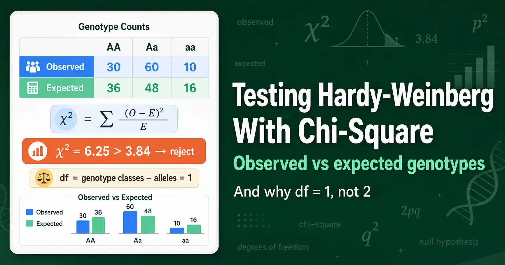
To test whether a population is in Hardy-Weinberg equilibrium, you use a chi-square test that compares the observed genotype counts to the counts expected under equilibrium. First calculate the allele frequencies from the observed data, then use p², 2pq, and q² to find the expected counts, and finally compute the chi-square statistic as the sum of (observed minus expected) squared, divided by expected, across all genotypes. For a two-allele gene, you compare the result to a critical value of 3.84, using one degree of freedom, not two.
The chi-square test turns Hardy-Weinberg from a prediction into a testable hypothesis, letting you decide statistically whether a real population departs from equilibrium. This guide walks through the full procedure with a worked example, and it explains the single most confusing part of the test: why the degrees of freedom for a two-allele system is 1 rather than 2. That detail trips up many students, and getting it right is what separates a correct test from a wrong one. The equilibrium predictions can be generated with a calculator before running the test by hand.
Why a Chi-Square Test Is Needed
Hardy-Weinberg gives you the genotype frequencies a population should have if it is in equilibrium. But real data never match a prediction perfectly, even when the population truly is in equilibrium, because of ordinary sampling variation. The question is whether the difference between what you observe and what you expect is small enough to be chance, or large enough to mean something real.
This is exactly the kind of question a chi-square goodness-of-fit test answers. The test takes your observed counts and your expected counts and produces a single number, the chi-square statistic, that measures how far the observations stray from the expectations. A small statistic means the observed and expected counts are close, consistent with equilibrium. A large statistic means they diverge more than chance comfortably allows, signaling that the population deviates from equilibrium and that some evolutionary force may be at work.
The logic is that of a null hypothesis test, which fits Hardy-Weinberg perfectly since the principle is itself a null model. The null hypothesis is that the population is in Hardy-Weinberg equilibrium. The chi-square test looks for evidence against that null. If the evidence is strong enough, you reject the null and conclude the population is not in equilibrium. If it is not, you fail to reject the null, meaning the data are consistent with equilibrium. This is the same chi-square machinery used to test Mendelian ratios in genetic crosses, applied here to whole-population genotype data. The underlying statistical method is covered in the context of crosses by the Mendelian ratio chi-square calculator.
Step 1: Count the Observed Genotypes
The test begins with real data: the observed number of individuals of each genotype in your sample. For a gene with two alleles, A and a, you count how many individuals are homozygous dominant (AA), how many are heterozygous (Aa), and how many are homozygous recessive (aa). These three counts are your observed values.
It is important that these are genotype counts, not phenotype counts. The chi-square test for Hardy-Weinberg compares genotype frequencies, so you need to be able to distinguish all three genotypes. This works directly when the gene shows codominance or incomplete dominance, where each genotype has its own phenotype, such as the MN blood group in humans where MM, MN, and NN are all distinguishable. When there is complete dominance, AA and Aa look the same, and you cannot count them separately by phenotype alone, which complicates the test. For this reason, chi-square tests of Hardy-Weinberg are usually done on genes where all three genotypes can be identified.
Suppose you sample 100 individuals for a codominant gene and find 30 AA, 60 Aa, and 10 aa. These are your observed counts, totaling 100 individuals. Hold on to them, because the entire test compares these observed numbers against the numbers Hardy-Weinberg predicts. The total sample size, 100 here, will be used to convert expected frequencies into expected counts in a later step. Always confirm your observed counts sum to your total sample size before proceeding.
Step 2: Calculate Allele Frequencies From the Data
Here is the step that makes a Hardy-Weinberg chi-square different from a simple ratio test, and it is the source of the degrees-of-freedom subtlety later. You must calculate the allele frequencies from your own observed data, because the expected counts depend on them.
Use the counting method on your observed genotypes. The frequency of the A allele, p, is the number of A alleles divided by the total number of alleles. With 30 AA and 60 Aa individuals, the A alleles number 2 times 30 plus 60, which is 120, out of 2 times 100, which is 200 total alleles. So p equals 120 divided by 200, which is 0.6. The frequency of the a allele, q, is 1 minus 0.6, which is 0.4, and you can confirm it directly: 2 times 10 plus 60, which is 80, divided by 200, also gives 0.4.
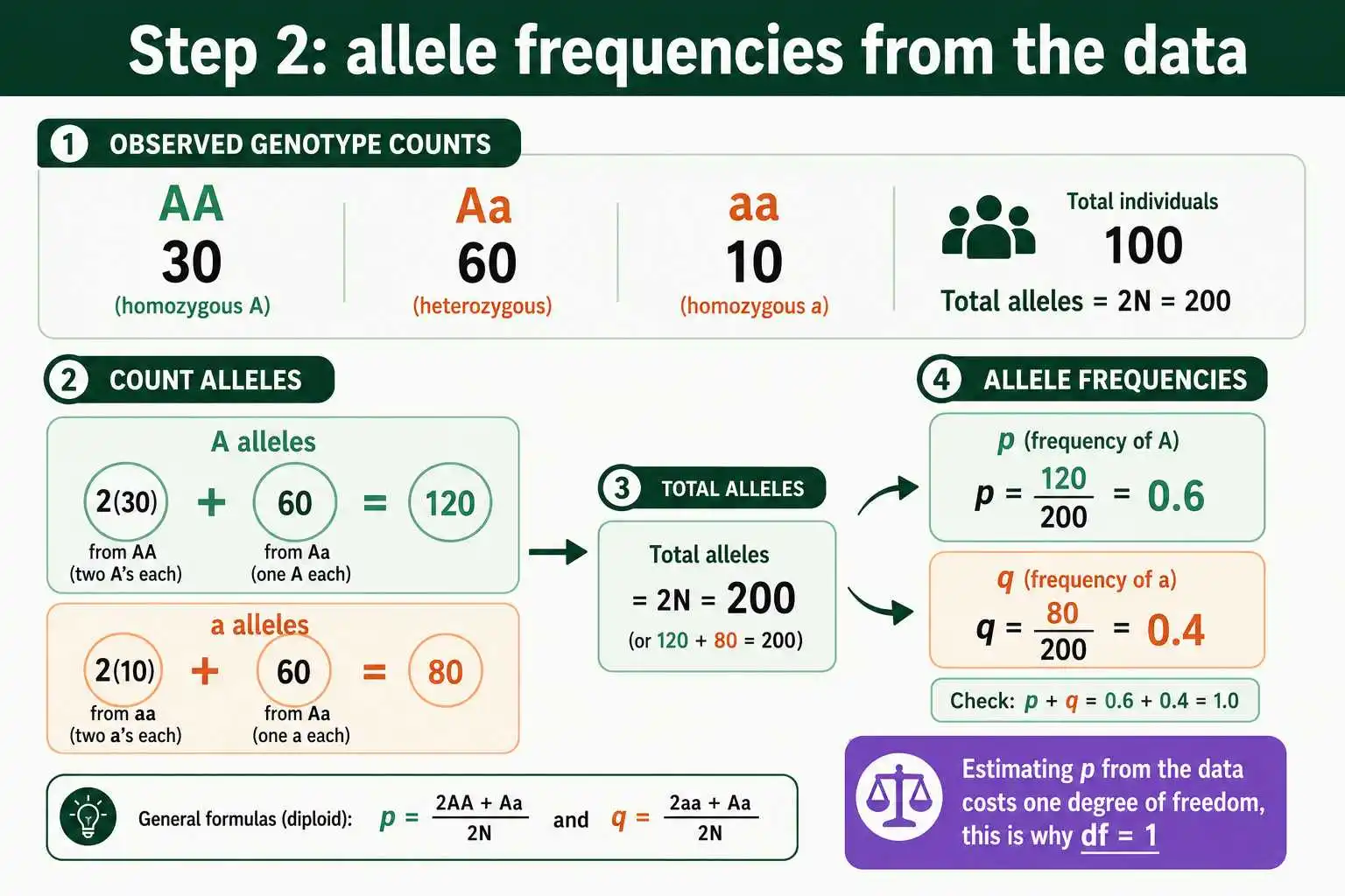
Notice what just happened: you used the observed data to estimate p and q. This is essential, because the expected genotype counts are built from these allele frequencies, but it has a statistical cost. By estimating a parameter from the data, you reduce the degrees of freedom by one, which is precisely why a Hardy-Weinberg chi-square ends up with one degree of freedom instead of two. The full method for finding allele frequencies from genotype counts is the standard counting approach, dividing the number of copies of each allele by the total number of alleles in the sample.
Step 3: Find the Expected Counts
With the allele frequencies in hand, you calculate the genotype frequencies Hardy-Weinberg predicts, then convert them to expected counts by multiplying by the sample size. These expected counts are what the population should look like if it is in equilibrium with the allele frequencies you measured.
Apply the Hardy-Weinberg genotype equation using p equals 0.6 and q equals 0.4. The expected frequency of AA is p², which is 0.36. The expected frequency of Aa is 2pq, which is 2 times 0.6 times 0.4, or 0.48. The expected frequency of aa is q², which is 0.16. These sum to 1, as they must. Now convert to expected counts by multiplying each frequency by the total sample size of 100. The expected count of AA is 0.36 times 100, which is 36. The expected count of Aa is 0.48 times 100, which is 48. The expected count of aa is 0.16 times 100, which is 16.
Lay the observed and expected counts side by side: AA observed 30 versus expected 36, Aa observed 60 versus expected 48, and aa observed 10 versus expected 16. The observed heterozygotes exceed the expected, while both homozygote classes fall short of their expected counts. Whether this difference is statistically meaningful is the question the chi-square statistic now answers. Always check that your expected counts sum to the same total as your observed counts, here both totaling 100, as a guard against arithmetic slips.
Step 4: Calculate the Chi-Square Statistic
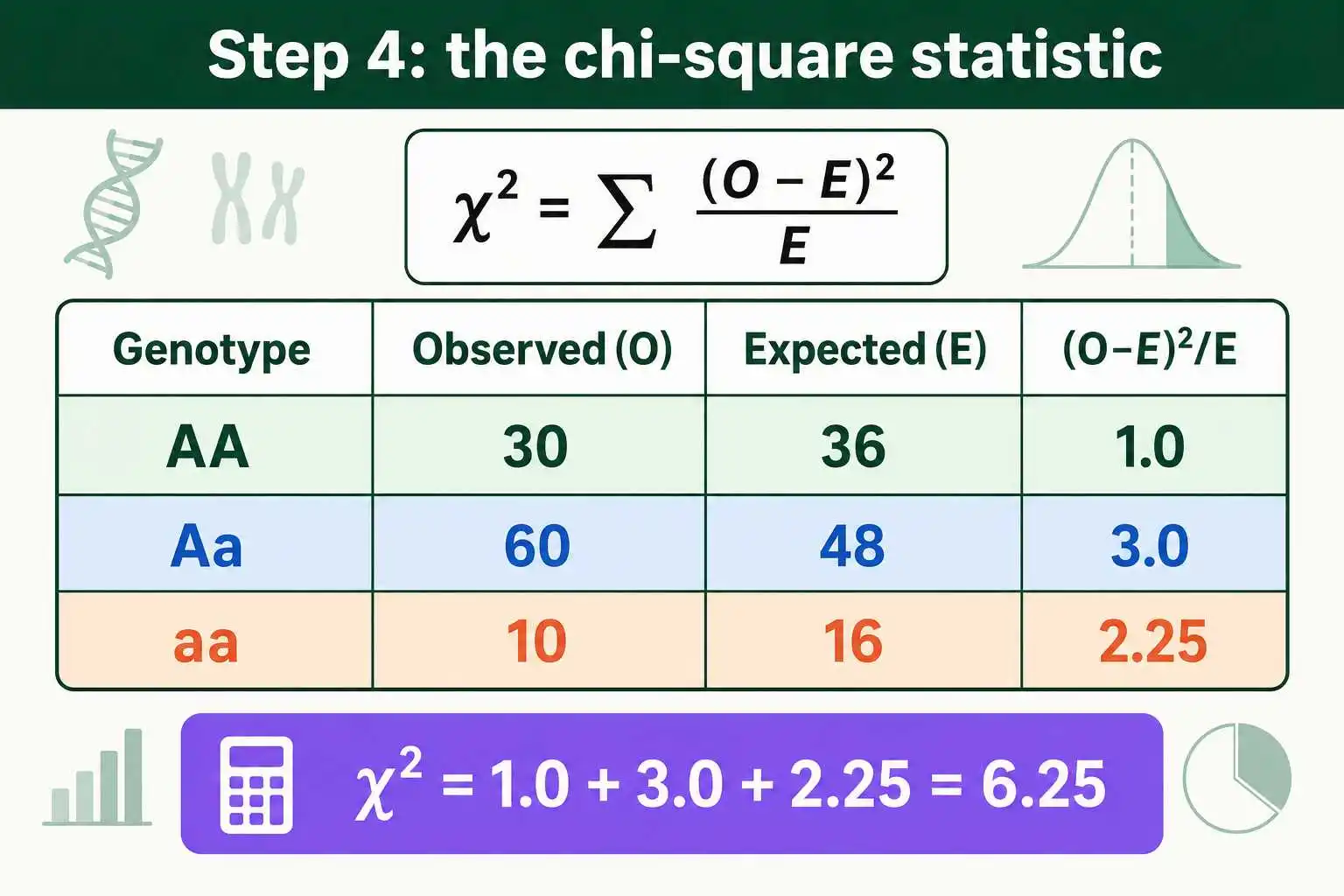
The chi-square statistic combines all the observed-versus-expected differences into one number. The formula is the sum, across all genotype classes, of the quantity observed minus expected, squared, then divided by expected. Squaring makes every difference positive and gives extra weight to larger gaps, and dividing by the expected count scales each difference relative to how big it should be.
Work through the three genotype classes with the numbers from the example. For AA, observed 30 minus expected 36 is negative 6, squared is 36, divided by 36 is 1.0. For Aa, observed 60 minus expected 48 is 12, squared is 144, divided by 48 is 3.0. For aa, observed 10 minus expected 16 is negative 6, squared is 36, divided by 16 is 2.25. Add these three contributions: 1.0 plus 3.0 plus 2.25 gives a chi-square statistic of 6.25.
This single value, 6.25, summarizes how far the whole population departs from the Hardy-Weinberg expectation. A value of zero would mean the observed counts matched the expected counts exactly. The larger the statistic, the greater the discrepancy. To interpret 6.25, you compare it against a critical value from the chi-square distribution, which requires knowing the degrees of freedom. That is the step where Hardy-Weinberg tests have their famous twist.
Step 5: Degrees of Freedom, the Tricky Part
The degrees of freedom for a Hardy-Weinberg chi-square with two alleles is 1, not 2, and understanding why is the key to doing the test correctly. This is the single most common error, because a naive count of categories suggests 2, and many students stop there.
In a standard goodness-of-fit test, the degrees of freedom is the number of categories minus 1. With three genotype categories, that rule alone would give 3 minus 1, which is 2. But the Hardy-Weinberg test has an extra subtraction, because you estimated the allele frequency p from the observed data itself. Every parameter you estimate from the data costs an additional degree of freedom. So the calculation is the number of genotype classes, 3, minus 1 for the usual sampling constraint, minus 1 more for estimating p, giving 3 minus 2, which is 1. The general formula is the number of genotype classes minus the number of alleles, which for two alleles is 3 minus 2, equal to 1.
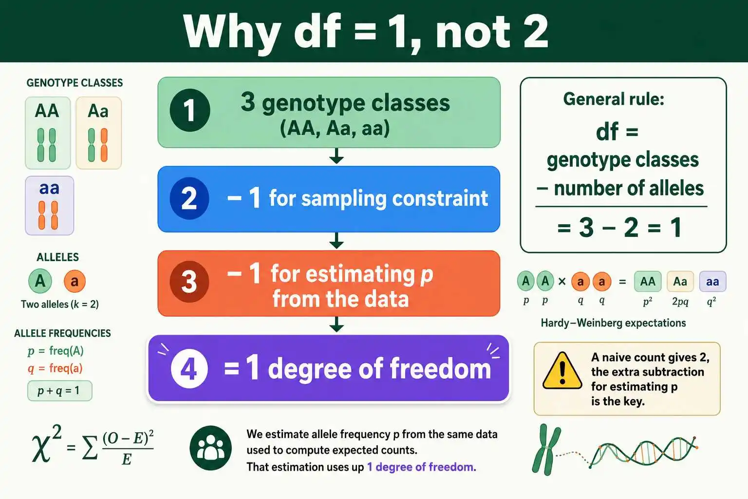
The reason estimating p costs a degree of freedom is that the expected counts were not fixed in advance; they were derived from the data. Different observed data would have given different allele frequencies and therefore different expected counts, so the expected values are not independent of the observations. You did not have to estimate q separately, because q is fully determined by p through p plus q equals 1, which is why only one parameter, not two, is subtracted. For a three-allele system the same logic gives 6 genotype classes minus 3 alleles, equal to 2 degrees of freedom, and the pattern continues for more alleles.
Step 6: Compare to the Critical Value and Conclude
The final step compares your chi-square statistic to the critical value for your degrees of freedom at a chosen significance level, conventionally 0.05. For one degree of freedom at the 0.05 level, the critical value is 3.84. This threshold is the dividing line between attributing the deviation to chance and concluding it is real.
The critical value comes from a chi-square distribution table, which lists the threshold for each combination of degrees of freedom and significance level. At one degree of freedom, the 0.05 critical value is 3.84, the 0.01 critical value is 6.63, and the 0.001 value is 10.83. Choosing a stricter significance level, like 0.01, raises the bar for declaring a deviation significant, reducing the chance of a false positive but making it harder to detect a real effect. The conventional 0.05 level balances these risks and is standard in most genetics work, which is why 3.84 is the number to remember for a two-allele Hardy-Weinberg test.
The decision rule is straightforward. If your chi-square statistic is less than the critical value, you fail to reject the null hypothesis, meaning the observed counts are consistent with Hardy-Weinberg equilibrium. If your statistic is greater than the critical value, you reject the null hypothesis and conclude that the population significantly deviates from equilibrium. In the worked example, the statistic is 6.25, which is greater than 3.84. So you reject the null hypothesis: this population is not in Hardy-Weinberg equilibrium for this gene.
What does that conclusion mean biologically? A significant deviation tells you that one or more of the Hardy-Weinberg conditions is being violated, so some evolutionary force, selection, drift, gene flow, mutation, or non-random mating, is likely acting on the population. The pattern in the example, an excess of heterozygotes and a shortage of homozygotes, hints at a possible cause such as heterozygote advantage or disassortative mating, though the test alone cannot identify which force is responsible. The chi-square result tells you that something is happening, and the direction of the deviation offers a clue, but pinning down the exact cause requires further investigation, as discussed in our guide on what disrupts Hardy-Weinberg equilibrium.
How This Differs From a Mendelian-Cross Chi-Square
Students often meet the chi-square test first in the context of Mendelian crosses, testing whether offspring fit an expected ratio like 3:1 or 9:3:3:1. The Hardy-Weinberg chi-square uses the same statistic but differs in one crucial way, and seeing the contrast clarifies the degrees-of-freedom rule.
In a Mendelian-cross chi-square, the expected ratio is fixed in advance by the genetic hypothesis. A monohybrid cross predicts 3:1 before you collect any data, so the expected counts come entirely from theory, not from the observations. With two phenotype classes and a predetermined ratio, the degrees of freedom is simply the number of classes minus 1, giving 2 minus 1, which is 1. Nothing is estimated from the data, so no extra degree of freedom is lost.
The Hardy-Weinberg chi-square is different because the expected counts are not fixed in advance. You have to estimate the allele frequencies from the very data you are testing, and only then can you calculate the expected genotype counts. This data-dependence is what costs the additional degree of freedom. So even though a Hardy-Weinberg test has three genotype classes, more than the two phenotype classes of a simple monohybrid test, both can end up with one degree of freedom, for entirely different reasons. The cross-based version of this test, with its theory-fixed ratios, is covered in our guide to chi-square analysis in AP Biology, and comparing the two cements when you do and do not subtract for estimated parameters.
Practical Cautions When Running the Test
A few practical considerations affect whether a Hardy-Weinberg chi-square gives trustworthy results, and being aware of them keeps your conclusions sound. The test is simple to compute, but its validity depends on some conditions being met.
The most important is sample size. The chi-square test is an approximation that works well only when the expected counts are reasonably large. A common rule of thumb is that every expected count should be at least 5; if any expected genotype count falls below that, the test becomes unreliable and the chi-square approximation breaks down. This often happens with rare recessive genotypes, where the expected q² count can be very small in a modest sample. In such cases, a larger sample or an exact test is needed. Always glance at your smallest expected count before trusting the result.
A second caution concerns interpretation rather than calculation. Failing to reject the null hypothesis does not prove the population is in equilibrium; it only means the data are consistent with equilibrium. A non-significant result might also occur because the sample was too small to detect a real deviation. Conversely, with a very large sample, even a biologically trivial deviation can become statistically significant. And as noted earlier, certain forces like balancing selection can leave a population looking close to equilibrium even when selection is active. The chi-square test is a powerful screening tool, but its results should be read with these limits in mind rather than treated as final proof either way. As one biology simulations resource notes, a population can sometimes display the expected Hardy-Weinberg data even while an evolutionary force is present, which is why a passing result is evidence of consistency rather than a guarantee of equilibrium.
Frequently Asked Questions
Why is the degrees of freedom 1 and not 2 for a Hardy-Weinberg chi-square?
Because you estimate the allele frequency p from the observed data, which costs an extra degree of freedom. The calculation is genotype classes minus alleles, so 3 minus 2 equals 1. A standard goodness-of-fit test would give 2, but estimating a parameter from the data subtracts one more.
What is the critical value for a Hardy-Weinberg chi-square test?
For a two-allele gene with one degree of freedom at the 0.05 significance level, the critical value is 3.84. If your chi-square statistic exceeds 3.84, you reject the hypothesis that the population is in equilibrium; if it is below, the data are consistent with equilibrium.
What does it mean if a population fails the Hardy-Weinberg test?
A significant deviation means one or more equilibrium conditions are violated, so an evolutionary force such as selection, drift, gene flow, mutation, or non-random mating may be acting. The test shows that something is changing the genotype frequencies, but it does not identify which force is responsible.
Do I use observed or expected counts in the chi-square formula?
Both. The formula is the sum of (observed minus expected) squared, divided by expected, for each genotype. You subtract expected from observed, square the result, then divide by the expected count, and add these up across all genotype classes to get the statistic.
From Prediction to Proof
Testing Hardy-Weinberg equilibrium with chi-square follows a clear sequence: count the observed genotypes, calculate allele frequencies from that data, use p², 2pq, and q² to find expected counts, compute the chi-square statistic as the summed squared differences over expected, then compare to the critical value of 3.84 using one degree of freedom. A statistic above 3.84 means the population significantly deviates from equilibrium.
The detail that matters most is the degrees of freedom: it is 1 for a two-allele gene, not 2, because estimating the allele frequency from the data costs an extra degree of freedom. Remembering the rule of genotype classes minus alleles keeps you from the most common mistake in the whole procedure. You can build the expected frequencies for any allele frequencies using the allele frequency calculator, then run the chi-square comparison by hand. For a clear worked treatment of the test with the statistical reasoning laid out, this EvoMath tutorial from The Panda's Thumb is a thorough reference.