How to Calculate Linkage Disequilibrium (D, D', r²)

To calculate linkage disequilibrium, you compare the observed frequency of a haplotype to the frequency expected if the two alleles were independent. The difference is D, the basic LD coefficient. From D you derive the two measures used in practice, D prime and r squared. That is the entire workflow.

This guide works through it with real numbers. It covers the D formula, why D needs normalizing, how to compute D prime and r squared, and a full worked example from haplotype counts to final values. If you need the concept behind the math first, our explainer on what linkage disequilibrium is sets it up.

Start With the Haplotype Frequencies

Every LD calculation begins with haplotype frequencies. For two loci with two alleles each, A/a and B/b, there are four possible haplotypes: AB, Ab, aB, and ab. You need the frequency of each.

Label them p_AB, p_Ab, p_aB, and p_ab. These four frequencies sum to one, because every chromosome carries one of the four combinations. From them you also get the individual allele frequencies: the frequency of A is p_AB plus p_Ab, and the frequency of B is p_AB plus p_aB. Everything else is derived from these numbers.

In practice, getting haplotype frequencies can take a step of its own, because genotype data does not always reveal which alleles sit together on the same chromosome. When the phase is unknown, software estimates haplotype frequencies using methods like expectation-maximization. But once you have the four haplotype frequencies, the LD math is straightforward arithmetic.

The Phasing Problem

The biggest practical hurdle in calculating LD is getting the haplotype frequencies in the first place. With unphased genotype data, you often cannot tell directly which alleles sit together on the same chromosome, and this complicates the starting point.

Consider an individual who is heterozygous at both loci, with genotype Aa at the first and Bb at the second. This person carries one of two possible haplotype pairs: either AB and ab, or Ab and aB. The genotype looks identical either way, so a single double-heterozygote does not reveal its phase. Across a sample, this ambiguity means the four haplotype frequencies cannot simply be counted.

The standard solution is the expectation-maximization algorithm, which estimates the most likely haplotype frequencies given the observed genotypes. It starts with a guess, computes the expected haplotype counts, updates the frequencies, and repeats until the values stabilize. Modern LD software does this automatically, which is why you can feed it genotype data and get D prime and r squared without resolving phase by hand. For teaching and for already-phased data, though, you work directly from the haplotype frequencies, as the examples here do. The key point is to know whether your starting frequencies are true counts or statistical estimates, because that affects how much to trust small LD values.

The D Coefficient

D is the difference between the observed frequency of a haplotype and the frequency expected under independence. It is the foundation of every LD measure.

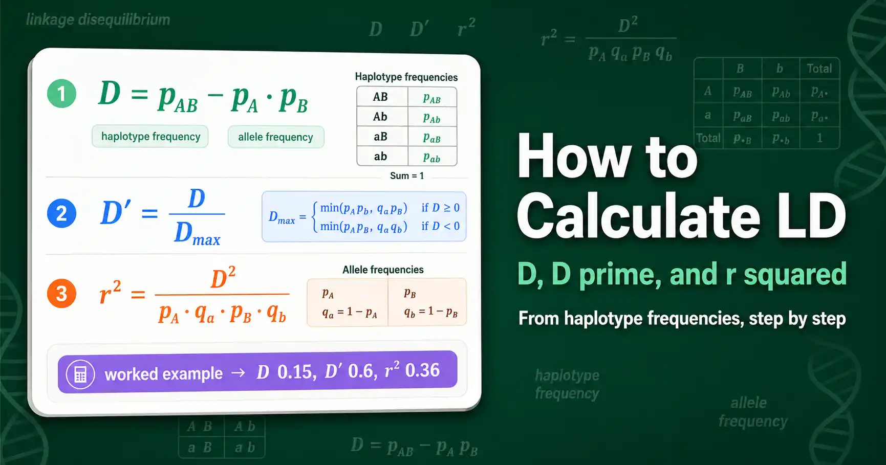
The formula is direct. D equals the frequency of the AB haplotype minus the product of the frequency of A and the frequency of B:

D = p_AB − (p_A × p_B)

There is an equivalent and often handier form using all four haplotypes:

D = (p_AB × p_ab) − (p_Ab × p_aB)

Both give the same number. When D is zero, the observed haplotype frequency matches the independent expectation, and the loci are in linkage equilibrium. When D is positive, AB and ab appear more than expected; when negative, Ab and aB do. The sign just reflects which allele combinations are over-represented, and is partly a matter of labeling. The D coefficient was defined by Richard Lewontin and Ken-ichi Kojima in their 1960 paper, the one that named linkage disequilibrium.

Why D Needs Normalizing

D has a serious limitation: its range depends on the allele frequencies, so the same D value can mean strong LD for one pair of loci and weak LD for another. This makes raw D values impossible to compare across locus pairs.

The problem is that D cannot reach its theoretical extremes unless the allele frequencies are equal. If one allele is rare, the maximum possible D is small, so a modest D might actually represent strong association. You cannot tell how strong the LD is from D alone without knowing the allele frequencies. This is why nobody reports raw D as a measure of LD strength.

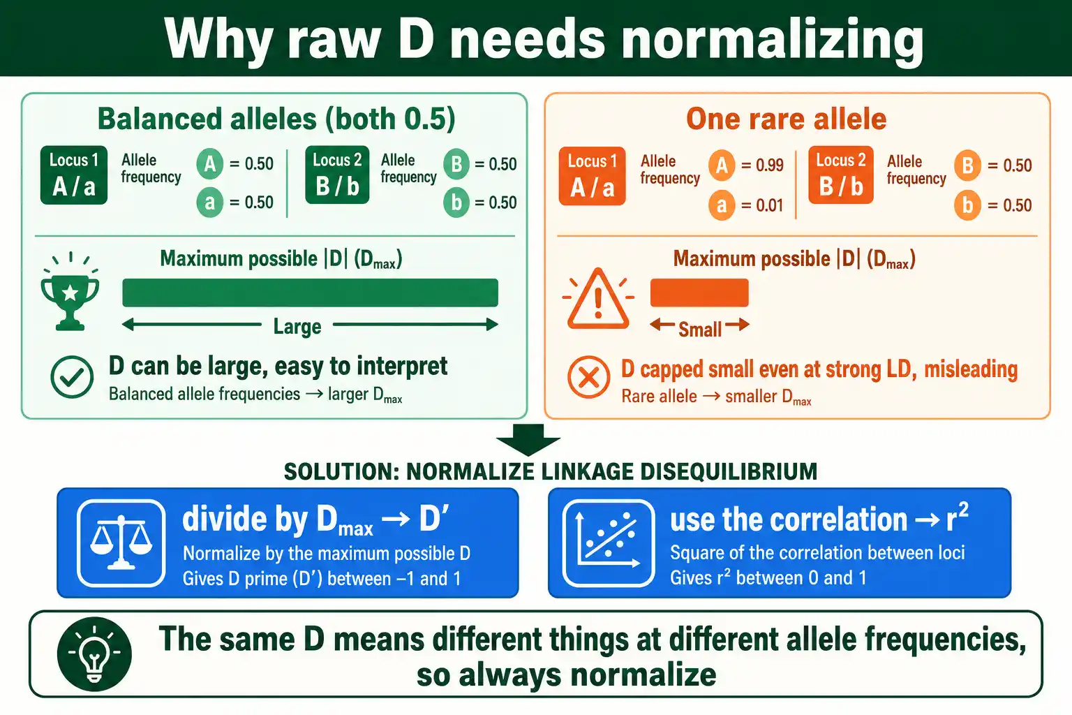
Two normalizations fix this, each in its own way. D prime rescales D against the maximum it could reach given the allele frequencies. R squared expresses the association as a squared correlation. Both convert the frequency-dependent D into a number you can interpret and compare, which is why they, not D, are what you actually report.

Calculating D Prime

D prime, introduced by Lewontin in 1964, divides D by its maximum possible value given the allele frequencies. The result runs from negative one to one, or from zero to one in absolute value.

The maximum depends on the sign of D. When D is positive, the maximum possible value is the smaller of two products: p_A times q_b, or q_a times p_B, where q denotes the alternative allele frequency. When D is negative, you use the smaller absolute value of p_A times p_B, or q_a times q_b. Then:

D' = D / D_max

The interpretation is clean. A D prime of one is called complete LD, and it means no recombination has yet separated the two loci in the sample, so at least one of the four possible haplotypes is missing entirely. A D prime below one means all four haplotypes are present, evidence that recombination has occurred between the loci. This is why D prime is the measure of choice for detecting historical recombination and mapping haplotype block boundaries.

Calculating r Squared

R squared is the squared correlation coefficient between the two loci, and it is the LD measure most used in modern genomics. It runs cleanly from zero to one. The measure traces to the work of William Hill and Alan Robertson in 1968, who developed the correlation framework for LD.

The formula divides D squared by the product of all four allele frequencies:

r² = D² / (p_A × q_a × p_B × q_b)

An r squared of zero means no association; the loci are independent. An r squared of one means perfect LD: the two loci are perfectly correlated, so knowing the allele at one locus tells you the allele at the other with certainty. In that case only two of the four haplotypes exist. Values in between measure how well one locus predicts the other.

This predictive quality is exactly why r squared dominates genome-wide association studies. When a marker SNP is in high r squared with a causal variant, the marker reliably stands in for it, which is the whole basis of tagging. The relationship between r squared and D prime, and when to use each, is the subject of our guide on D prime versus r squared.

A Full Worked Example

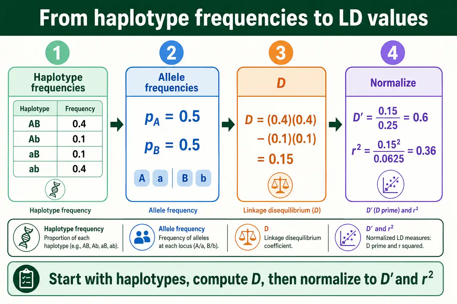
Put it all together with numbers. Suppose you sample chromosomes at two loci and observe these four haplotype frequencies: AB at 0.4, Ab at 0.1, aB at 0.1, and ab at 0.4.

First, the allele frequencies. The frequency of A is p_AB plus p_Ab, which is 0.4 plus 0.1, or 0.5. So q_a is also 0.5. The frequency of B is p_AB plus p_aB, which is 0.4 plus 0.1, or 0.5, making q_b 0.5 as well. Both loci have evenly balanced alleles.

Now D, using the four-haplotype form: D equals p_AB times p_ab, minus p_Ab times p_aB. That is 0.4 times 0.4, minus 0.1 times 0.1, which is 0.16 minus 0.01, giving D equals 0.15. Because D is positive and sizable relative to these frequencies, there is clear LD.

Next D prime. Since D is positive, D_max is the smaller of p_A times q_b, or q_a times p_B. Both are 0.5 times 0.5, which is 0.25, so D_max is 0.25. Then D prime equals 0.15 divided by 0.25, which is 0.6. That is moderate-to-strong LD, with all four haplotypes still present.

Finally r squared. The denominator is p_A times q_a times p_B times q_b, which is 0.5 times 0.5 times 0.5 times 0.5, or 0.0625. Then r squared equals D squared, 0.15 times 0.15 is 0.0225, divided by 0.0625, which is 0.36. So the two loci share 36 percent of their variation. You can check any set of haplotype frequencies against these formulas with a tool that computes D, D prime, and r squared automatically.

A Second Example: Unequal Frequencies

The first example had balanced allele frequencies, which kept D prime and r squared in rough agreement. They diverge sharply when one allele is rare, and a second example shows why this matters.

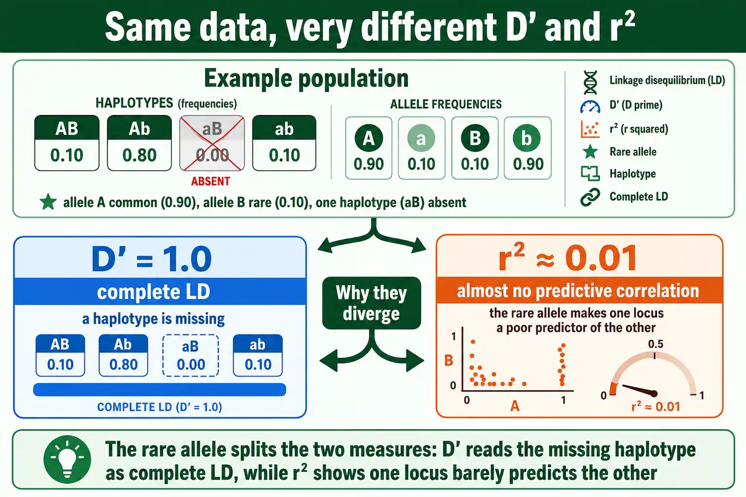
Suppose the haplotype frequencies are AB at 0.45, Ab at 0.05, aB at 0.05, and ab at 0.45, but now imagine instead a case where allele A is common and allele B is rare. Take AB at 0.10, Ab at 0.80, aB at 0.00, and ab at 0.10. The allele frequencies are: A is 0.10 plus 0.80, or 0.90; B is 0.10 plus 0.00, or 0.10. So A is common and B is rare.

Compute D: p_AB times p_ab minus p_Ab times p_aB, which is 0.10 times 0.10 minus 0.80 times 0.00, giving 0.01 minus 0, or D equals 0.01. Now D prime. Since D is positive, D_max is the smaller of p_A times q_b, which is 0.90 times 0.90, or 0.81, and q_a times p_B, which is 0.10 times 0.10, or 0.01. The smaller is 0.01, so D_max is 0.01, and D prime equals 0.01 divided by 0.01, which is one. Complete LD: the aB haplotype is entirely absent.

Now r squared: D squared is 0.0001, and the denominator is p_A times q_a times p_B times q_b, which is 0.90 times 0.10 times 0.10 times 0.90, or 0.0081. So r squared equals 0.0001 divided by 0.0081, which is about 0.012, nearly zero. The same locus pair gives D prime of one and r squared near zero. The reason is the rare allele: one haplotype is missing, which D prime reads as complete LD, but the rare allele means one locus still barely predicts the other, which is what r squared measures. This divergence is the single most important thing to understand about the two measures.

Reading the Three Numbers Together

The worked example produced three numbers from one dataset: D of 0.15, D prime of 0.6, and r squared of 0.36. Each says something slightly different, and reading them together is the skill.

D of 0.15 tells you the raw excess of the AB and ab haplotypes over independence, but on its own it is hard to judge without the allele frequencies. D prime of 0.6 tells you the loci are well short of complete LD, so recombination has produced all four haplotypes, but substantial association remains. R squared of 0.36 tells you one locus predicts the other moderately well, capturing about a third of the variation.

In a real report, you would lead with D prime or r squared depending on the question. For historical recombination and haplotype structure, D prime is the headline. For predictability and tagging, r squared is. D itself is the engine under the hood, rarely reported directly but always the starting point. Knowing all three keeps you from misreading any one of them in isolation.

There is also a quick sanity check the three numbers give you together. R squared can never exceed D prime squared, so if you ever compute an r squared larger than D prime, you have made an arithmetic error somewhere. And when allele frequencies at the two loci are similar, D prime and r squared move close together, while a large gap between them is a reliable flag that one allele is rare. Reading the spread between D prime and r squared, not just their individual values, often tells you more about the locus pair than either number alone, because that spread encodes how balanced the allele frequencies are.

Is the LD Statistically Significant?

A computed D prime or r squared does not tell you, on its own, whether the LD is real or a fluke of sampling. For that, you test it, and the test matters most when samples are small.

The standard significance test for LD is a chi-square test. It compares the observed haplotype frequencies against those expected under linkage equilibrium, and a large chi-square value, with a correspondingly small p-value, means the association is unlikely to be due to chance. Conveniently, the chi-square statistic for a two-locus, two-allele table equals r squared times the sample size of chromosomes, which links the strength measure directly to the significance test. A larger sample makes a given r squared more significant.

This is why sample size is part of any honest LD report. A high D prime from a handful of chromosomes can be an artifact, because small samples easily produce missing haplotypes by chance, inflating D prime toward one. The same is true of LD estimated from unphased data, where the haplotype frequencies are themselves estimates. The practical rule is to report the sample size alongside the LD measures, and to lean on r squared and its significance test rather than D prime when samples are small, because D prime is the more easily inflated of the two. Strength and significance are different questions, and a complete answer gives both.

Common Calculation Mistakes

A few errors trip people up. Watching for them keeps your LD values correct.

The first is forgetting that haplotype frequencies, not genotype frequencies, drive the calculation. LD is about which alleles sit together on the same chromosome, so you need phased haplotypes or estimated haplotype frequencies, not just counts of genotypes. Mixing these up produces wrong values.

The second is reading raw D as a measure of strength. Because D's range depends on allele frequencies, a small D can mean strong LD when an allele is rare. Always normalize to D prime or r squared before judging how strong the association is.

The third is confusing the two normalized measures. D prime and r squared answer different questions and can differ sharply for the same data, especially when allele frequencies are unequal. A high D prime with a low r squared is common and not a contradiction, a point worth understanding before comparing values. The fourth is sign confusion: the sign of D depends on which alleles you label as the reference, so the magnitude matters more than whether D comes out positive or negative.

Frequently Asked Questions

What is the formula for linkage disequilibrium?

The basic measure is D, defined as D equals the frequency of the AB haplotype minus the product of the frequencies of allele A and allele B. Equivalently, D equals p_AB times p_ab minus p_Ab times p_aB. From D you compute D prime, by dividing by its maximum possible value, and r squared, by dividing D squared by the product of all four allele frequencies.

How do you calculate r squared for LD?

Divide D squared by the product of the four allele frequencies: r² equals D² divided by p_A times q_a times p_B times q_b. The result runs from zero, meaning no association, to one, meaning perfect correlation between the two loci. R squared is the LD measure most used in genome-wide association studies.

What does a D prime of 1 mean?

A D prime of one is called complete linkage disequilibrium. It means at least one of the four possible haplotypes is absent, so no recombination has yet separated the two loci in the sample. A D prime below one means all four haplotypes are present, indicating recombination has occurred between the loci.

From Haplotypes to a Number

Calculating LD follows one path: start with the four haplotype frequencies, compute D as the gap between observed and expected, then normalize. D prime rescales D against its maximum to reveal recombination history, and r squared expresses the association as a squared correlation that measures predictability. The worked example carried one dataset through all three, from D of 0.15 to D prime of 0.6 and r squared of 0.36.

The practical takeaway is to normalize before interpreting and to read all three numbers together, since each captures a different facet of the same association. To see how that association is generated and broken down over time, our guide on LD decay and recombination traces the forces behind the numbers, and our explainer on what causes linkage disequilibrium covers what builds LD in the first place.