Linkage Disequilibrium in GWAS Explained
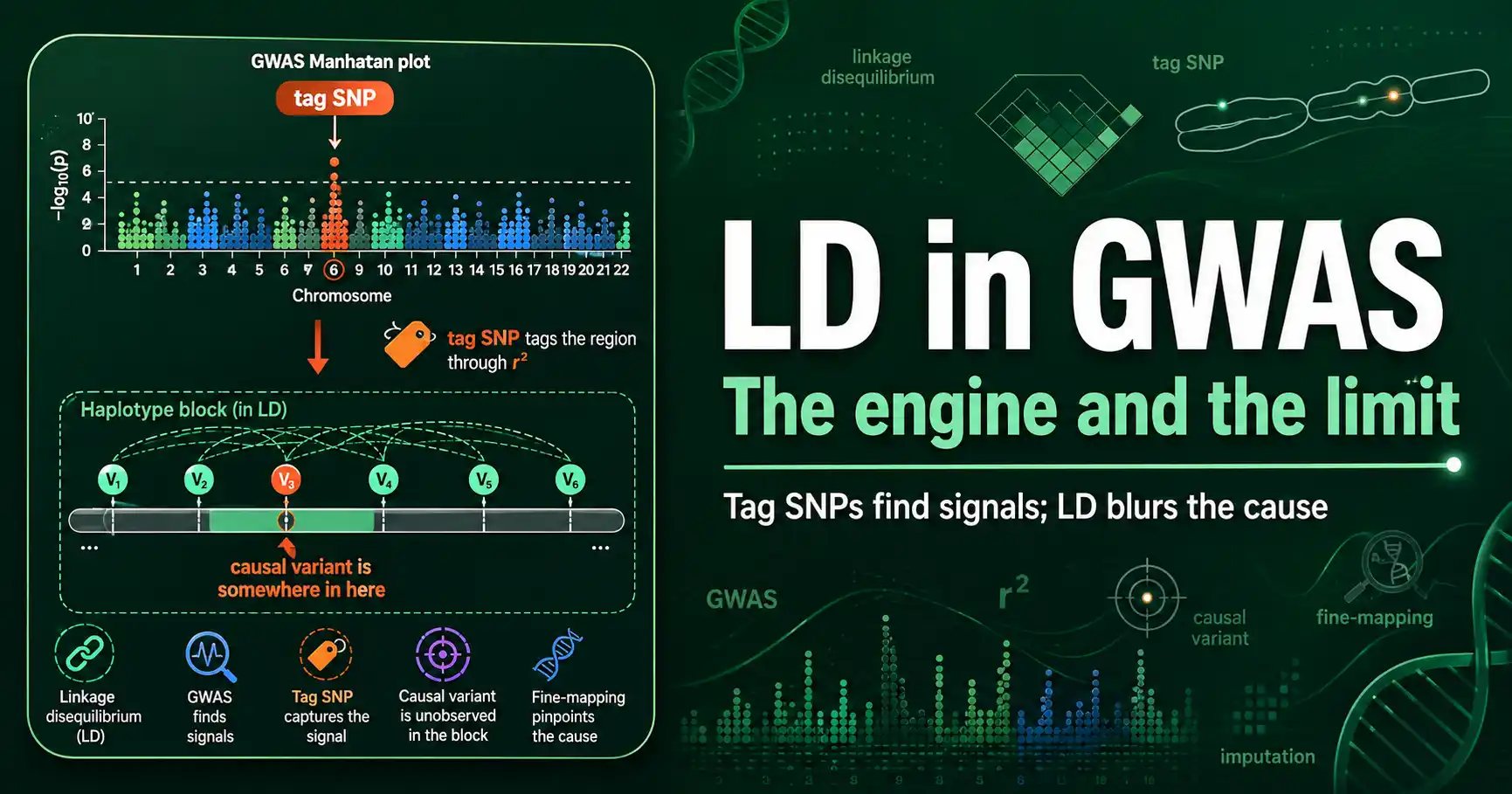
Linkage disequilibrium is what makes genome-wide association studies work. Because nearby variants are correlated through LD, genotyping a few hundred thousand marker SNPs captures variation across the whole genome, and a marker associated with a disease points to a nearby causal variant. The same LD that gives GWAS its power also creates its central limitation: an associated marker is rarely the cause itself, just a flag for the neighborhood.
This guide explains how LD drives modern human genetics. It covers tag SNPs, why association hits are not automatically causal, fine-mapping, imputation, and the cross-ancestry portability problem that LD creates for polygenic scores. For the foundation, our explainer on what linkage disequilibrium is sets it up.
Why GWAS Depends on LD
A genome-wide association study tests whether genetic variants are associated with a trait or disease. There are tens of millions of common variants in the human genome, far too many to genotype individually in the large samples GWAS needs. LD is what makes the problem tractable.
Because variants close together sit in haplotype blocks of strong LD, they are highly correlated, so you do not need to type every one. A few hundred thousand well-chosen marker SNPs capture most of the common variation, because each marker is in LD with the untyped variants around it. This is the principle of tagging: a genotyped tag SNP stands in for the variants it is correlated with. Without LD, every causal variant would have to be genotyped directly, and genome-wide studies at scale would be impossible.
The measure that matters here is r squared, the squared correlation between loci, because it quantifies how well one variant predicts another. A tag SNP with high r squared to a causal variant captures its signal well; one with low r squared misses it. The distinction between r squared and the other main LD measure is covered in our guide on D prime versus r squared.
Tag SNPs and Statistical Power
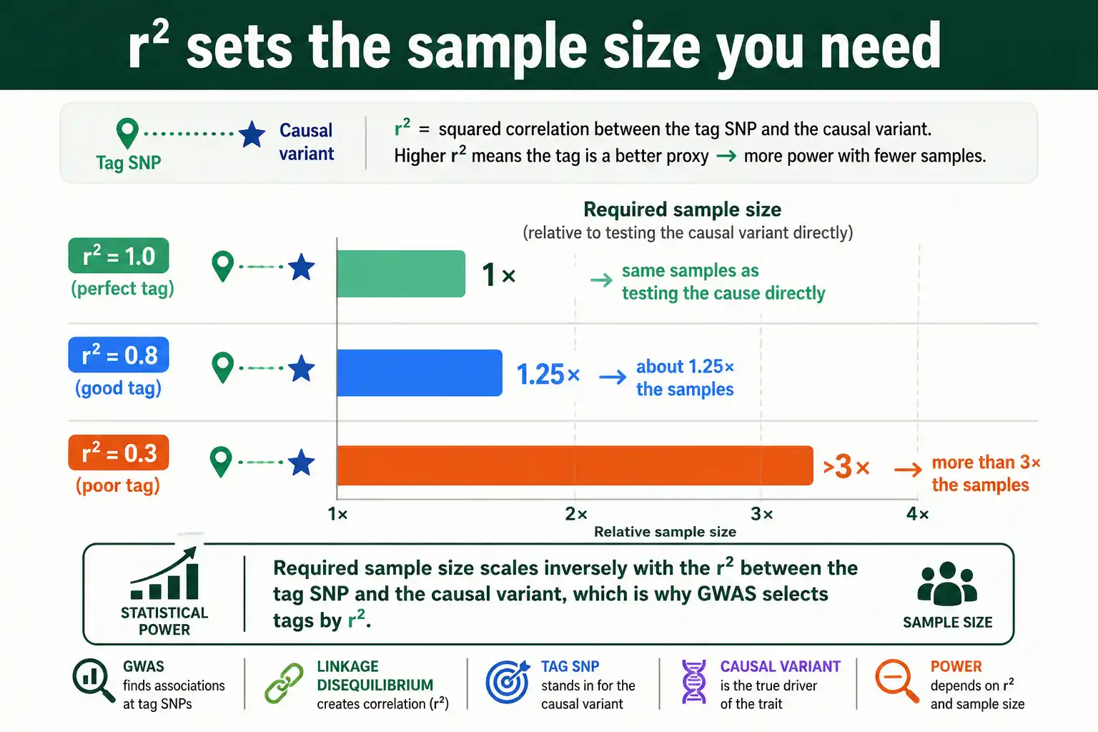
The reason r squared is the right measure for GWAS comes down to statistical power, and the relationship is precise. The sample size needed to detect an association through a tag SNP scales inversely with the r squared between the tag and the causal variant.
In practice this means a tag SNP in perfect LD with a causal variant, r squared of one, needs no more samples than genotyping the causal variant directly. A tag with r squared of 0.5 needs twice the sample size to reach the same power. A tag with r squared of 0.2 needs five times as many. So the strength of LD between markers and causal variants directly sets how powerful, and how expensive, a study must be.
This is why tag SNP selection became a science of its own. Choosing a marker set that maximizes r squared with the untyped variants, while minimizing the number of markers, is what made early genome-wide studies affordable. You can see how haplotype frequencies translate into the r squared that governs tagging by working through the LD between two markers. The same logic carries into newer designs, where dense reference data lets a modest genotyping array capture the genome through LD.
Why Association Hits Are Not Always Causal
The defining catch of GWAS is that an associated marker is usually not the causal variant, just a variant in LD with it. This is the single most important thing to understand about interpreting GWAS results.
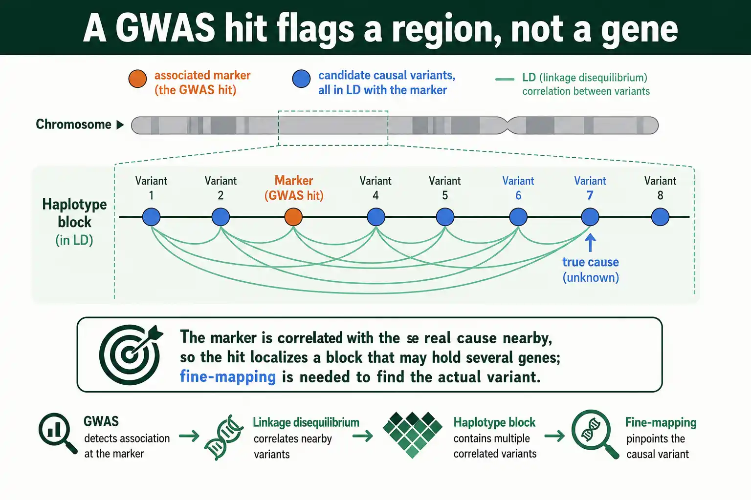
When a study finds a SNP associated with a disease, that SNP is flagged because it is correlated with the true causal variant nearby, not necessarily because it does anything itself. The causal variant might be any of dozens of variants in the same haplotype block, all in strong LD with the associated marker and with each other. As Jonathan Pritchard and Molly Przeworski emphasized in a 2001 review of linkage disequilibrium in humans, the estimated effect of any SNP reflects its LD with the actual causal sites, so a marker can show a strong association while being biologically inert.
This is why a GWAS hit defines a region, not a gene. The associated marker localizes the signal to a haplotype block that may contain several genes and many variants. Turning that region into a specific causal variant requires further work, because LD that helped find the signal now blurs its exact source. The blurring is the price of the power: the same correlations that let a few markers scan the genome prevent those markers from resolving the cause precisely.
Fine-Mapping: From Region to Cause
Fine-mapping is the process of narrowing a GWAS-associated region down toward the actual causal variant. It is necessary precisely because LD spreads the association signal across many correlated variants.
The core idea is to use the LD structure itself to rank candidates. Statistical fine-mapping methods combine the association strengths with the LD pattern to produce a credible set: the smallest group of variants likely to contain the true causal one, with attached probabilities. A tight credible set means LD in the region is broken up enough to localize the cause; a broad one means strong LD leaves many variants indistinguishable. Studies of fine-mapping precision have found that the causal variant usually lies within about 100 kilobases of the genome-wide significant marker, and in strong LD with it, which bounds the search.
Fine-mapping also draws on outside information to break LD ties. Functional data, which variants sit in regulatory regions, which affect protein sequence, which influence gene expression, helps prioritize the biologically plausible candidates among the statistically indistinguishable ones. And because LD differs between populations, combining data across ancestries can narrow a credible set, since a causal variant stays associated everywhere while the markers merely tagging it through population-specific LD do not. This is one place where the diversity of LD patterns becomes an asset rather than an obstacle.
The intuition for cross-ancestry fine-mapping is worth spelling out. A true causal variant affects the trait in every population, so it shows association wherever it is common. A marker that is only tagging the causal variant does so through the local LD pattern, which differs by population, so its association strength changes from one group to another. By overlaying association signals from several populations, researchers can spot the variant whose signal is consistent everywhere, the causal one, and downweight the markers whose apparent effect shifts with the local LD. The shorter-range LD of African-ancestry populations is especially valuable here, because it breaks large haplotype blocks into smaller pieces, letting fine-mapping resolve a credible set that European-ancestry data alone, with its longer blocks, would leave blurred. This is a concrete scientific reason, beyond equity, that diversifying genomic data improves the science for everyone.
Imputation: Filling In Untyped Variants
Genotype imputation uses LD to infer variants that were never directly measured. It is one of the most powerful routine applications of LD in genetics.
The method works by comparison to a reference panel: a densely sequenced set of haplotypes, such as those from large sequencing projects. A study that genotyped only a few hundred thousand markers can be compared against the reference, and because the study samples share haplotype structure with the reference, the untyped variants can be filled in statistically from the surrounding typed markers and the known LD. This boosts a sparse genotyping array up to tens of millions of variants without sequencing every sample.
Imputation has two big payoffs. It lets studies test far more variants than they genotyped, increasing the chance of capturing causal variants, and it lets separate studies be combined by imputing all of them to the same variant set, which is what makes the huge meta-analyses behind modern GWAS possible. The accuracy of imputation depends on how well the reference panel's LD matches the study population's, which is why reference panels strive to include diverse ancestries. A poorly matched panel imputes poorly, foreshadowing the portability problem below.
Imputation accuracy also falls off for rare variants, and the reason is again LD. Common variants sit in well-characterized haplotype patterns that the reference panel captures reliably, so they impute well. Rare variants appear on fewer reference haplotypes and are in weaker r squared with surrounding common markers, so the surrounding genotypes carry less information about them, and imputation is correspondingly less certain. This is why studies chasing rare causal variants increasingly turn to direct sequencing rather than relying on imputation, and why ever-larger and more diverse reference panels are built: a bigger panel contains more copies of each rare haplotype, improving the LD information available to impute the rare variants that matter most for some diseases.
LD Clumping and Pruning
Before and after the association test, LD is used to clean up the marker set, through two related procedures called pruning and clumping. Both prevent correlated markers from distorting results.
LD pruning thins a dense marker set down to a roughly independent subset by removing markers in high LD with others, keeping one representative from each correlated group. This matters for analyses that assume independent markers, like principal-component analysis of population structure or estimates of genome-wide relatedness, because leaving in many correlated markers would overweight whatever the cluster of markers happens to tag. Pruning gives those methods the near-independent input they expect.
LD clumping does the complementary job on association results. After a GWAS, many neighboring markers show association simply because they are in LD with the same underlying signal, so the raw list of hits double-counts each real signal many times. Clumping groups the hits around the strongest marker in each LD region, collapsing a cluster of correlated associations into one representative signal. The result is a clean list of independent association signals rather than a redundant pile of correlated ones. Both procedures rest on the same insight that drives the rest of GWAS: markers are correlated through LD, and that correlation must be accounted for rather than ignored. The independence that pruning and clumping approximate is the same independence assumed by Hardy-Weinberg equilibrium at a single locus, extended here to the relationship between loci.
A Worked Tagging Example
A concrete tagging case shows why r squared, not D prime, sets GWAS power. Suppose a causal variant for a disease sits in a haplotype block, untyped, and a nearby marker SNP is genotyped instead.
If that marker has an r squared of 0.8 with the causal variant, it captures most of the causal variant's statistical signal, so a study using the marker needs only about 1 divided by 0.8, roughly 1.25 times, as many samples as it would need testing the causal variant directly. That is a small penalty, and the marker is an excellent tag. If instead the marker has an r squared of 0.3 with the causal variant, the study needs about 1 divided by 0.3, more than three times as many samples to reach the same power. Same physical distance, very different consequences, because r squared captures the predictive correlation that power depends on.
This is also why a marker with high D prime but low r squared, the rare-allele case, makes a poor tag despite looking strongly associated by one measure. A study that selected tags by D prime could include this marker, expect it to capture the causal signal, and end up badly underpowered. The worked logic is the practical reason GWAS pipelines select and evaluate tags by r squared specifically.
The Cross-Ancestry Portability Problem
LD creates a serious equity problem in human genetics: polygenic scores built in one population predict poorly in another, largely because LD patterns differ between populations. This is one of the most consequential practical issues LD raises.
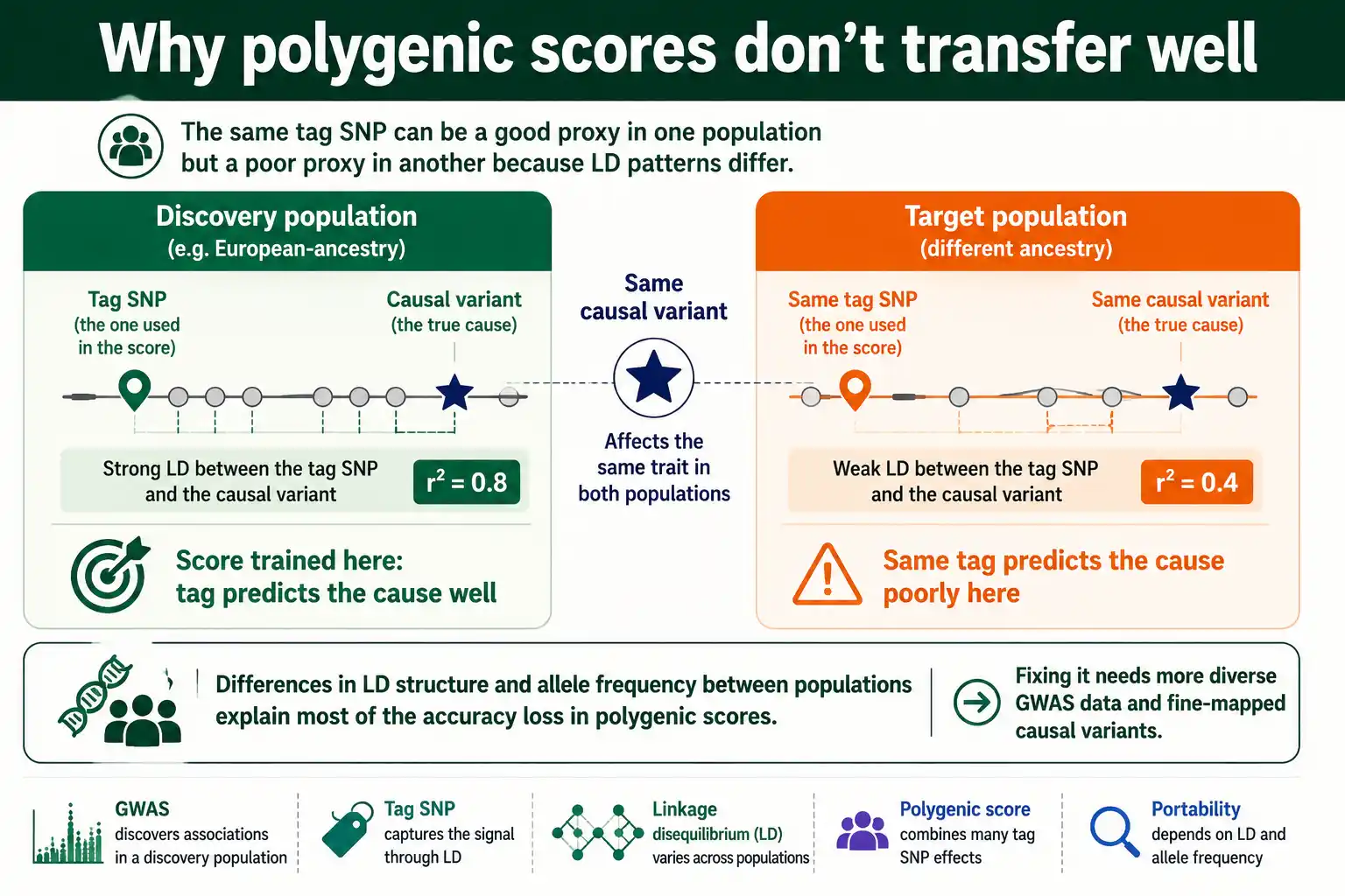
A polygenic score sums the effects of many variants to predict a trait or disease risk. But those effects are estimated through tag SNPs, whose predictive value depends on their LD with the true causal variants. Because LD patterns differ across populations with different demographic and recombination histories, a tag SNP that strongly predicts a causal variant in one population may predict it weakly in another. So a score trained mostly in European-ancestry samples loses accuracy when applied to people of other ancestries. As Alicia Martin and colleagues documented in an influential 2019 paper in Nature Genetics, this portability gap risks turning genomic medicine into a source of health inequity, because the great majority of GWAS data has come from European-ancestry populations.
The cause is specific and well-studied. One analysis estimated that differences in LD and in allele frequencies between populations together account for 70 to 80 percent of the loss of polygenic-score accuracy from European to African samples. The fixes all involve LD: assembling more diverse GWAS data so scores can be trained with population-appropriate LD, fine-mapping causal variants so prediction relies less on population-specific tagging, and developing methods that explicitly model LD differences. The portability problem is, at its root, an LD problem, and solving it is a major priority for making genomic medicine equitable.
How LD Is Used in GWAS: A Summary
LD threads through every stage of a genome-wide study. The table collects the main uses.
| Stage | How LD is used |
|---|---|
| Study design | Tag SNPs capture untyped variants through LD, cutting genotyping cost |
| Statistical power | Required sample size scales inversely with r² between tag and causal variant |
| Quality control | LD clumping and pruning remove redundant correlated markers |
| Interpreting hits | Associated marker tags a region; the causal variant lies nearby in LD |
| Fine-mapping | LD structure defines credible sets of candidate causal variants |
| Imputation | LD with a reference panel infers untyped genotypes |
| Polygenic scores | Differing LD across populations limits cross-ancestry portability |
The table shows a single theme running through GWAS: LD is simultaneously the enabler and the complication. It makes the genome scannable with a manageable marker set, and it blurs the precise cause of every signal those markers find. Mastering GWAS is largely a matter of using LD's power while managing its blur.
Frequently Asked Questions
Why are GWAS hits not always the causal variant?
Because GWAS detects markers in linkage disequilibrium with the true causal variant, not necessarily the causal variant itself. An associated marker is flagged because it is correlated with the real cause nearby, so the causal variant could be any of many variants in the same haplotype block. This is why a GWAS hit identifies a region, and fine-mapping is needed to localize the actual cause.
What is a tag SNP?
A tag SNP is a genotyped marker chosen to stand in for many nearby untyped variants through linkage disequilibrium. Because variants in a haplotype block are correlated, a single tag SNP with high r squared to its neighbors captures their variation, letting a few hundred thousand markers represent the common variation across the genome. This is the basis of efficient genome-wide genotyping.
Why do polygenic scores work less well across ancestries?
Mainly because linkage disequilibrium patterns differ between populations. Polygenic scores rely on tag SNPs whose predictive value depends on their LD with causal variants, and since LD differs across populations with different histories, a score trained in one population predicts less accurately in another. Differences in LD and allele frequency are estimated to explain most of the accuracy loss between populations.
LD: The Engine and the Limit of GWAS
Linkage disequilibrium is the foundation of genome-wide association studies. It lets a manageable set of tag SNPs scan the entire genome, because each marker is correlated with the variants around it, and the required sample size scales inversely with the r squared between a tag and its causal variant. That same correlation means a GWAS hit tags a region rather than pinpointing a cause, which is why fine-mapping, using LD structure and functional data to define credible sets, is needed to localize the actual variant.
LD also powers imputation, filling in untyped variants from a reference panel, and it lies behind the cross-ancestry portability problem, where differing LD patterns limit how well polygenic scores transfer between populations. The through-line is that LD is both the engine and the limit of modern human genetics: the correlations that make the genome searchable are the same ones that blur every answer. To revisit how these LD patterns arise and decay in the first place, our guides on what causes linkage disequilibrium and LD decay and recombination trace the forces behind the patterns GWAS exploits.