What Is Fst? Population Differentiation Explained
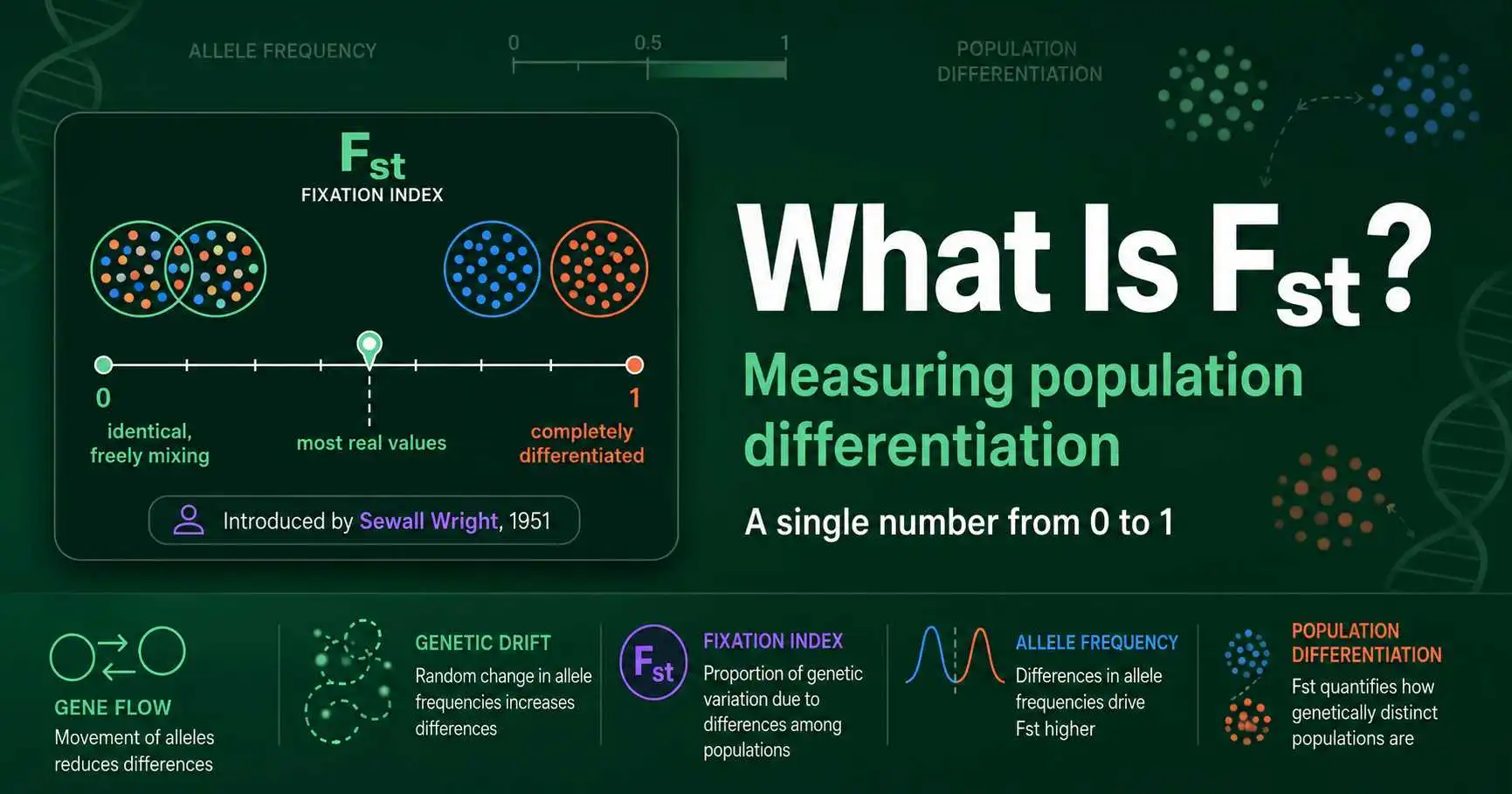
Fst is a number that tells you how genetically different two or more populations are. It runs from 0 to 1. A value of 0 means the populations are genetically identical, mixing so freely that they behave as one. A value of 1 means they are completely differentiated, sharing none of their genetic variation. Almost every real comparison falls somewhere in between, and that in-between number is what makes Fst so useful.
The full name is the fixation index, and it sits among the most widely used statistics in all of population genetics. Sewall Wright introduced it in 1951 as one of his F-statistics, and biologists have leaned on it ever since to ask a deceptively simple question: when a species is split into groups, how much of its genetic variation is due to differences between those groups rather than differences within them?
That question turns out to matter almost everywhere. Conservation biologists use Fst to decide whether two populations of an endangered animal are distinct enough to manage separately. Human geneticists use it to study ancestry and migration. Ecologists use it to map how gene flow moves across a landscape. This guide explains what Fst actually measures, where the idea came from, and how to interpret a value once you have one. A dedicated calculator can compute it for your own data once you understand what the number means.
The Core Idea: Variation Within Versus Between
Here is the heart of it. Take a species and split it into subpopulations. Some of the total genetic variation will exist as differences among individuals inside each subpopulation. The rest will exist as differences between the subpopulations themselves. Fst is the fraction of total variation that falls into that second category.
When subpopulations are nearly identical, almost all the variation is within them, and very little is between them. Fst is close to 0. When subpopulations have diverged, a larger share of the variation is accounted for by the differences between them, and Fst climbs toward 1. So Fst is really a ratio: between-population variation divided by total variation.
It helps to anchor this in a question you could actually ask. Pick a random pair of individuals from the whole species and a random pair from within one subpopulation. If the within-subpopulation pair tends to be just as genetically different as the species-wide pair, there is no structure, and Fst is near zero. If individuals within a subpopulation are noticeably more alike than two individuals drawn from the species at large, the subpopulations have pulled apart, and Fst rises to reflect the gap. That comparison, similarity inside groups versus similarity overall, is the intuition underneath every formula that follows.
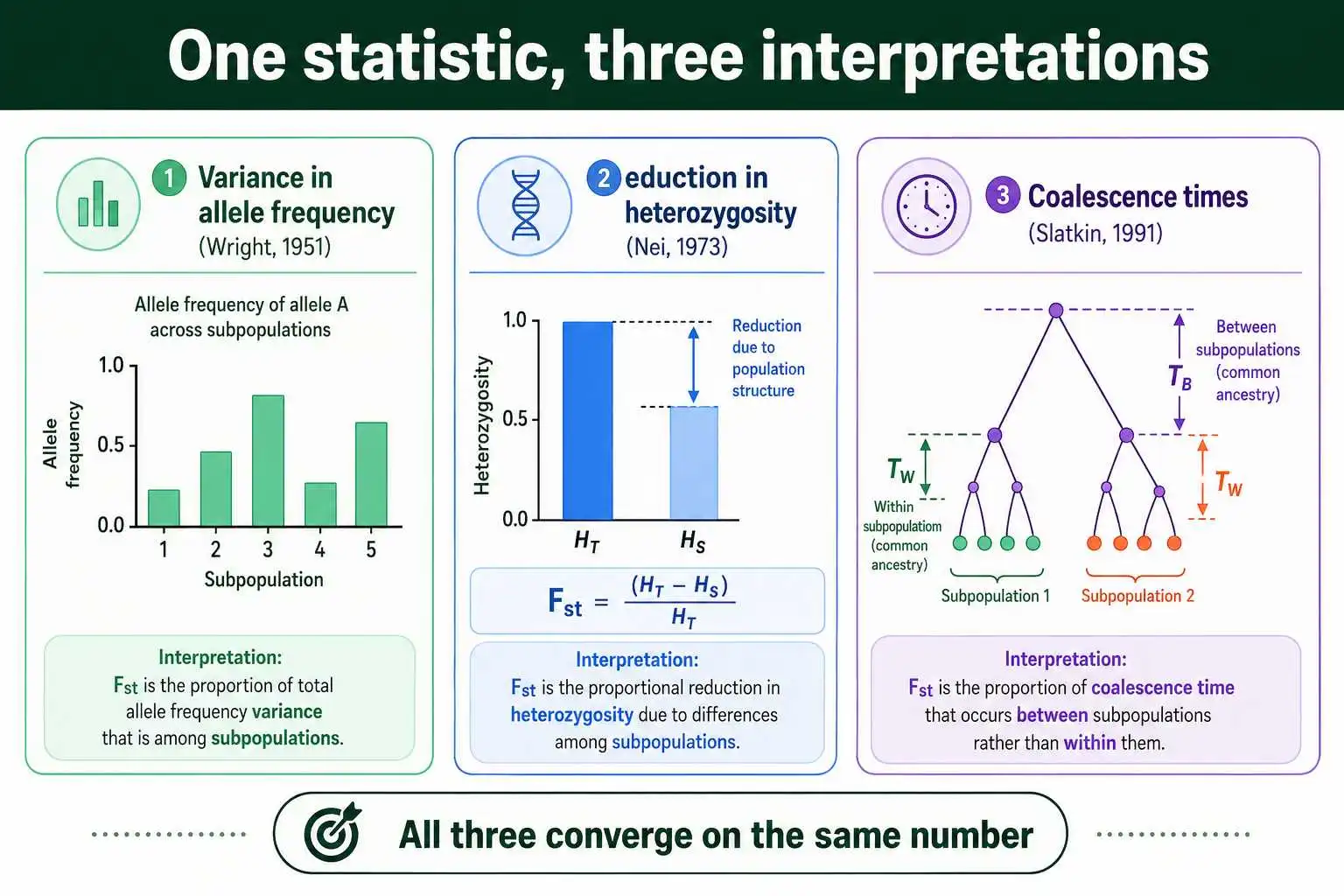
Wright framed this in terms of variance in allele frequencies. If you track a single allele, its frequency varies from one subpopulation to the next. Fst captures how large that variance is, relative to the maximum it could possibly be given the overall allele frequency. A later and equivalent way to express the same idea, developed by Masatoshi Nei in 1973, uses heterozygosity instead of variance, which many people find more intuitive.
Two Ways to Write It Down
Nei's version is worth seeing, because it makes the logic concrete. Define the expected heterozygosity of the whole population, pooling everyone together, as HT. Define the average expected heterozygosity within the subpopulations as HS. Then:
Fst = (HT − HS) / HT
Read that slowly. HT is how much genetic diversity you would expect if the whole species mated at random as one big pool. HS is how much diversity actually sits inside the subpopulations on average. If subdivision has caused the subpopulations to lose diversity relative to the whole, HS will be smaller than HT, and the gap between them, scaled by HT, is Fst. No subdivision means HS equals HT, the numerator is zero, and Fst is zero. Complete subdivision drives HS toward zero and Fst toward 1.
Wright's original variance definition and Nei's heterozygosity definition describe the same underlying quantity from different angles. Both appear constantly in the literature, and a paper might use either depending on the author's framework. Montgomery Slatkin added a third interpretation in 1991, framing Fst through coalescent theory as a comparison of how far back in time you have to go to find common ancestors within a subpopulation versus across the whole population. As Kent Holsinger and Bruce Weir put it in their 2009 review in Nature Reviews Genetics, the richness of Fst comes precisely from the fact that it can be derived and understood through several distinct theoretical frameworks, all of which converge on the same statistic.
Where the Statistic Came From
Sewall Wright was one of the three architects of the modern synthesis in evolutionary biology, alongside Ronald Fisher and J.B.S. Haldane. Among his lasting contributions are the F-statistics, a family of related measures he developed across the 1940s and crystallized in a 1951 paper, "The genetical structure of populations." Fst is the member of that family concerned with differentiation between subpopulations.
The "F" originally stood for fixation, the process by which an allele drifts to a frequency of 100 percent. Wright's insight was that population structure and inbreeding both increase the chance that the two alleles in an individual are identical, and his F-statistics quantify that increase at different levels: within individuals, within subpopulations, and across the whole population. Fst specifically measures the effect attributable to the subdivision itself.
For decades, Fst was estimated with Wright's straightforward formula applied directly to observed allele frequencies. The trouble, recognized by the 1980s, is that this estimator is biased when samples are small, because the noise of sampling inflates the apparent differences between groups. In 1984, Bruce Weir and C. Clark Cockerham published an estimator in the journal Evolution that recast the problem in the language of analysis of variance, partitioning genetic variation into components and correcting for sample size. Their estimator, often written as θ (theta), became the standard in practice, and it is what most modern software actually computes when it reports an "Fst." The mechanics of running that calculation, including how θ corrects for sample size, are laid out step by step in our guide on how to calculate Fst.
Fst's Two Siblings
Fst rarely travels alone. Wright defined three F-statistics together, and seeing the whole set clarifies what Fst is and is not.
The first is Fis, the inbreeding coefficient within subpopulations. It measures how far the individuals inside a subpopulation deviate from random mating, comparing the heterozygosity actually observed to what random mating within that group would produce. A positive Fis means fewer heterozygotes than expected, the signature of inbreeding or assortative mating inside the group.
The second is Fst, the differentiation among subpopulations, the subject of this article.
The third is Fit, the overall inbreeding coefficient of an individual measured against the total population, which combines the other two. All three obey one tidy relationship: (1 − Fit) = (1 − Fis)(1 − Fst). In words, the total deficit of heterozygosity an individual carries stacks two contributions, the non-random mating inside its own group and the differentiation between groups. That decomposition is why Fst is best understood as the between-group slice of a larger accounting of where heterozygosity goes when a species is subdivided. A practical upshot is that you can have substantial Fst with no inbreeding inside any group, or heavy inbreeding within groups that are barely differentiated from each other, since the two coefficients measure genuinely separate things. The within-group slice, Fis, connects to the logic behind the inbreeding coefficient.
Reading a Value
Suppose you run the numbers and get an Fst of 0.08. What does that tell you?
It tells you that 8 percent of the total genetic variation in your sample is explained by differences between the populations, and the other 92 percent by differences within them. That is a modest level of differentiation, the kind you might see between regional populations of a widespread species that still exchange some migrants. Wright himself offered rough qualitative guideposts, suggesting that values from 0 to 0.05 indicate little differentiation, 0.05 to 0.15 moderate differentiation, 0.15 to 0.25 great differentiation, and above 0.25 very great differentiation. These bands are conventions, not laws, and they shift with the organism and the markers used, but they give a starting sense of scale. Where these thresholds come from and how much to trust them is the subject of our closer look at what counts as a high or low Fst value.
A few cautions are worth carrying. Fst is sensitive to how diverse the underlying marker is, a problem that becomes severe for highly polymorphic markers like microsatellites, where the maximum possible Fst can be well below 1, making a "low" value misleading. Lou Jost argued in a 2008 paper in Molecular Ecology that this property makes Fst a poor measure of differentiation in some settings, sparking a long and productive debate that produced alternative statistics. Fst is also not a true distance in the mathematical sense, since it does not always satisfy the triangle inequality. None of this makes it useless; it makes it a tool whose assumptions you need to know.
What Drives Fst Up or Down
Two opposing forces set the value of Fst, and understanding them explains most of what you will ever see in real data.
Genetic drift pushes Fst up. In any finite population, allele frequencies wander randomly from generation to generation, and isolated subpopulations wander independently, drifting apart from one another. The smaller the subpopulations, the faster they diverge, so drift steadily increases differentiation over time when populations are separated.
Gene flow pulls Fst down. When migrants move between subpopulations and breed, they carry alleles with them, mixing the gene pools and erasing the differences that drift creates. Even a small amount of migration is a powerful homogenizing force. Wright captured this balance in his island model, which yields the well-known approximation that Fst is roughly 1 divided by the quantity 4Nm plus 1, where Nm is the number of migrants exchanged per generation. The takeaway from that formula is simple and almost counterintuitive: it implies that just a handful of migrants per generation, regardless of total population size, is enough to keep subpopulations from differentiating much. Plug in one migrant per generation and Fst settles near 0.2; raise it to five migrants and Fst drops to about 0.05. Because the formula depends on the number of migrants rather than the migration rate, even a vast population can be held together genetically by a trickle of movement. When Nm is large, Fst approaches 0; when Nm is small, drift wins and Fst climbs.
Mutation and selection can also shape Fst, though usually more subtly. Local adaptation, where different alleles are favored in different environments, can drive Fst at particular genes far above the genome-wide background, and scanning for these outlier loci is now a standard way to hunt for genes under selection. The relationship between differentiation, drift, and migration is taken up in more depth in our discussion of genetic differentiation and gene flow.
A Quick Worked Sense-Check
Imagine two populations of a flower. In population one, a red-petal allele has a frequency of 0.7. In population two, it has a frequency of 0.3. Pool them and the average frequency is 0.5.
Within each population, the expected heterozygosity is 2pq. For population one that is 2 times 0.7 times 0.3, or 0.42. For population two it is 2 times 0.3 times 0.7, also 0.42. So HS, the average within-population heterozygosity, is 0.42. For the pooled population with an allele frequency of 0.5, HT is 2 times 0.5 times 0.5, which is 0.5. Now apply Nei's formula: Fst equals (0.5 − 0.42) divided by 0.5, which is 0.08 divided by 0.5, giving 0.16.
An Fst of 0.16 signals fairly strong differentiation, which fits, because a swing from 0.7 to 0.3 in allele frequency is a large one. The arithmetic here is deliberately simple, but it mirrors exactly what the estimators do on real, multi-locus, multi-allele data: compare the diversity you see within groups to the diversity in the whole, and report the shortfall as a proportion.
What People Actually Do With It
The abstract definition comes alive in how researchers use Fst across fields, and a few concrete uses show its range.
In conservation, Fst helps decide management units. If two populations of a threatened species show high Fst, they have diverged enough that conservationists may treat them as separate units worth protecting individually, rather than freely mixing them. Low Fst suggests they function as one connected population. The northern hairy-nosed wombat, the Florida panther, and countless fish stocks have all been assessed this way, and the logic feeds directly into decisions about whether to attempt translocation between populations.
In the study of humans, Fst became a flashpoint for one of the most important findings in the field. Richard Lewontin, in a 1972 paper, partitioned human genetic variation and found that the overwhelming majority of it, roughly 85 percent, exists within populations rather than between them, with only a small fraction attributable to differences among major geographic groups. Human Fst across continental groups typically lands near 0.10 to 0.15, a modest value, and large genomic datasets have confirmed the basic pattern Lewontin described. Estimates from the 1000 Genomes Project and earlier HapMap data, for example, put Fst between European and East Asian samples at roughly 0.11.
In molecular ecology and evolution, Fst scans across the genome have become a workhorse for finding genes under local adaptation. The idea, refined by researchers including Mark Beaumont and others in the early 2000s, is that most of the genome drifts and migrates as a background, producing a baseline Fst, while a gene under divergent selection between environments will stand out as an Fst outlier far above that background. This outlier approach has flagged genes for everything from altitude adaptation to coat color, turning a single summary statistic into a search engine for natural selection.
Three Things Fst Is Not
A surprising amount of confusion around Fst comes from expecting it to be something it isn't. Three clarifications head off the most common mistakes.
It is not a measure of how "different" two populations look or behave. Fst tracks neutral genetic variation, the kind that drifts and flows without being pushed by selection. Two populations can look strikingly different in a few visible traits driven by a handful of selected genes while having a genome-wide Fst near zero, and the reverse can happen too. Visible difference and genome-wide differentiation are simply not the same thing.
It is not fixed for a pair of populations regardless of method. The number you get depends on the estimator, the markers, and the sampling. Wright's direct formula, Nei's Gst, and the Weir and Cockerham θ can return noticeably different values from the same data, especially with small samples or highly variable markers. Reporting which estimator produced a value is not pedantry; it is necessary for the number to mean anything to another researcher.
And it is not, by itself, a verdict on whether populations are "really" distinct. Fst is one input into questions about population structure, taxonomy, and conservation units, but those questions also draw on geography, ecology, behavior, and other genetic patterns. A single Fst value is a summary, not a conclusion. Treating it as the last word, rather than a well-defined piece of evidence, is where interpretation tends to go wrong.
A Worked Sense-Check, Extended
Return for a moment to that flower example, where two populations had red-allele frequencies of 0.7 and 0.3 and produced an Fst of 0.16. It is worth seeing what would change the answer.
Shrink the difference between the populations, say to 0.6 and 0.4, and HS rises toward HT, so Fst falls. Run the numbers: each population's heterozygosity is 2 times 0.6 times 0.4, or 0.48, so HS is 0.48, while the pooled frequency is still 0.5 and HT is still 0.5. Now Fst is (0.5 − 0.48) over 0.5, which is 0.04, a quarter of the previous value. A smaller frequency gap means less differentiation, exactly as intuition demands.
Push the populations fully apart instead, to 1.0 and 0.0, and every individual in population one carries the red allele while none in population two does. Within-population heterozygosity collapses to zero, so HS is 0, while the pooled frequency of 0.5 keeps HT at 0.5. Fst becomes (0.5 − 0) over 0.5, which equals 1, complete differentiation. These two extremes bracket everything Fst can report, and walking a single allele between them is the fastest way to build a feel for the scale.
Why It Endures
More than seventy years after Wright defined it, Fst remains the first number population geneticists reach for when they want to know how structured a species is. New sequencing technologies have only widened its use, since a single statistic that summarizes differentiation across thousands of genetic markers is exactly what genome-scale data calls for. The estimator has been refined, critiqued, and supplemented, but the underlying question Wright posed has never gone out of date.
The reason it endures is that the question is fundamental. Every species is, to some degree, a collection of partially separated populations, and how separated they are determines how the species evolves, how it should be conserved, and how its history can be read from its genes. Fst puts a number on that separation.
It also endures because it scales. A statistic invented to be computed by hand from a handful of blood-group frequencies in the 1950s turns out to work just as well summarizing differentiation across millions of single-nucleotide polymorphisms from a sequencing run. Few tools built in the pre-computer era have survived the genomic flood so gracefully. That durability is a sign that Wright captured something real about how variation is organized in nature, not merely a convenient bookkeeping device. To move from the concept to working with actual numbers, the natural next step is to try it on real allele frequencies with the Fst population differentiation calculator.