Fst Values Explained: What Counts as High or Low?

You have an Fst value. Now what does it mean? On its own, a number like 0.08 or 0.15 says nothing meaningful until you place it against some established sense of scale. The good news is that decades of accumulated data have built up that scale, both as rough qualitative bands and as a large library of real values measured in actual species. The harder news is that "high" and "low" depend heavily on what you are studying, so the same number can be unremarkable in one context and genuinely notable in another.
This guide gives you the benchmarks. It lays out Wright's classic interpretive bands, fills them in with real Fst figures drawn from humans and a wide range of other organisms, and explains the traps that make a raw value misleading. If you are still firming up the underlying concept itself, our explainer on what Fst is covers the foundation in detail. Here, the focus is purely on reading the number once you have it.
Wright's Classic Bands
The most widely cited yardstick comes from Sewall Wright himself, who in his 1978 work offered rough qualitative thresholds for interpreting Fst. They remain the default reference point in textbooks and papers, later codified in reviews such as François Balloux and Nicolas Lugon-Moulin's 2002 survey in Molecular Ecology.
Wright's guidelines break the 0-to-1 range into four bands. An Fst from 0 to 0.05 indicates little genetic differentiation. From 0.05 to 0.15 is moderate differentiation. From 0.15 to 0.25 is great differentiation. And anything above 0.25 represents very great differentiation. So a value of 0.08 sits in the moderate band, while 0.20 would count as great.
A caution comes attached to these numbers, and Wright himself understood it. The bands are conventions, not biological laws. They were never meant as hard cutoffs, and what counts as a notable Fst genuinely varies with the organism, the markers, and the question. Treating 0.05 or 0.15 as a magic line is exactly the kind of overreading the next sections are meant to prevent. The bands are a starting orientation, useful precisely because they are rough.
It also helps to know where the bands came from. Wright did not derive them from a statistical threshold; he proposed them as descriptive labels based on his experience with the organisms and datasets of his era, largely livestock and natural populations studied with the limited markers then available. Modern genomic data, with millions of markers, can detect statistically significant differentiation at Fst values far below 0.05, levels Wright would have called negligible. So a very low but reliably measured Fst can still be biologically real and useful, even though it falls in the "little differentiation" band. The bands describe magnitude, not statistical significance, and the two are not the same thing.
| Fst range | Wright's interpretation |
|---|---|
| 0 to 0.05 | Little differentiation |
| 0.05 to 0.15 | Moderate differentiation |
| 0.15 to 0.25 | Great differentiation |
| Above 0.25 | Very great differentiation |
What Real Values Look Like Across Species
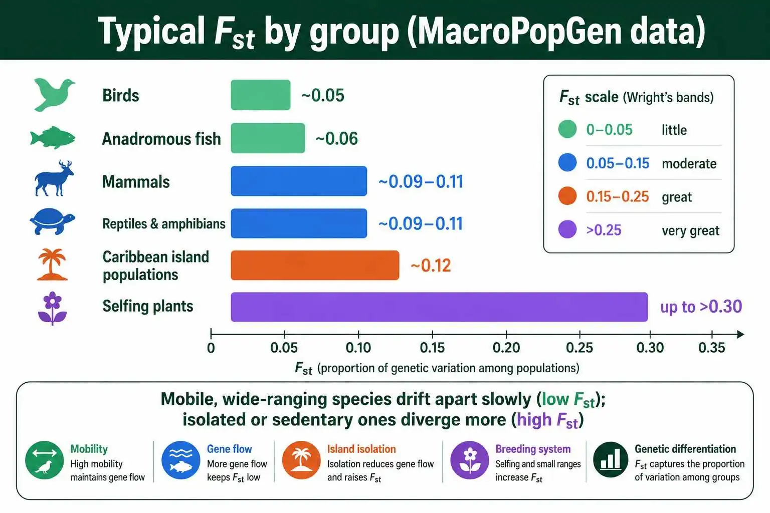
Bands are abstract. Real numbers from real organisms give a much better feel for what is typical, and a large body of comparative data now exists. One of the most comprehensive resources is the MacroPopGen database, compiled by researchers led by Jared Grummer and published in Scientific Data, which assembled Fst measurements from 1,308 microsatellite studies covering 897 vertebrate species across the Americas.
The patterns in that database are revealing. Birds had the lowest average differentiation, with a mean Fst around 0.05, and anadromous fishes such as salmon were nearly as low at about 0.06. The reason is mobility: animals that move widely and breed across large ranges exchange genes freely, which keeps Fst low. Less mobile groups showed more structure, with mammals, reptiles, amphibians, and freshwater fishes clustering in the 0.09 to 0.11 range. Caribbean island populations stood out at around 0.12, higher than mainland populations, exactly as island isolation would predict.
These figures sketch a general rule of thumb. Highly mobile, wide-ranging species tend toward low Fst because gene flow homogenizes them. Sedentary species, or those fragmented across islands and isolated habitats, tend toward higher Fst because drift pulls their subpopulations apart. A value of 0.10 is fairly ordinary for a mammal but would be strikingly high for a far-ranging seabird. Context, in other words, is built into what counts as high.
The same database revealed finer patterns worth noting. Heterozygosity stayed broadly similar across the vertebrate groups, ranging only from about 0.57 to 0.63, even though their Fst values differed substantially, a reminder that within-population diversity and between-population differentiation are separate quantities. Caribbean populations not only showed higher Fst but also carried fewer alleles on average than mainland groups, the expected signature of island isolation reducing both connectivity and diversity at once. Plants, not covered in that particular vertebrate database, often show higher Fst still, because many have limited seed and pollen dispersal and can self-fertilize, both of which restrict gene flow. Wind-pollinated trees tend toward lower plant values, while selfing herbs can reach Fst well above 0.3, among the highest routinely seen in nature.
Fst in Human Populations
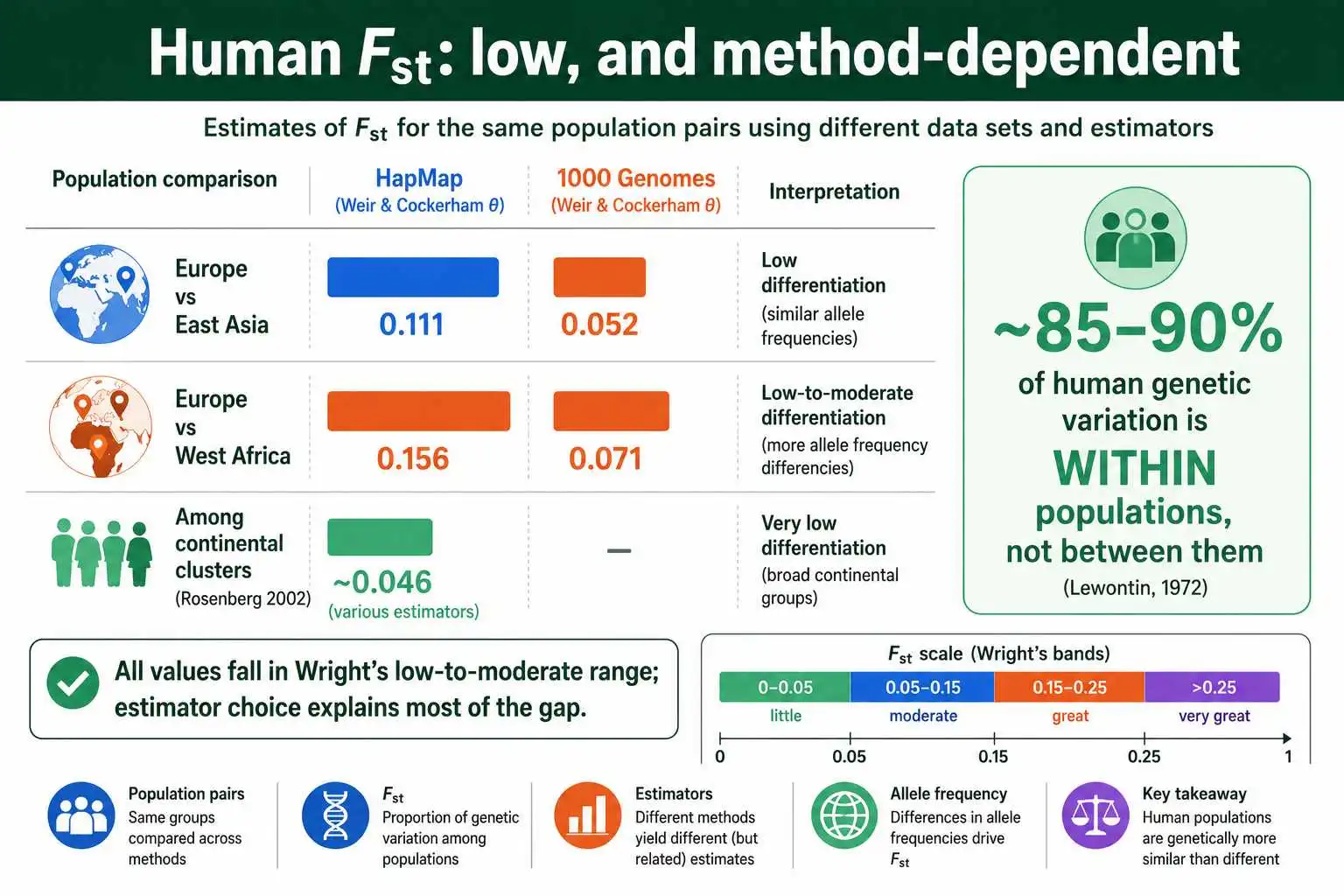
Human Fst is one of the most studied and most misunderstood figures in all of population genetics, so it deserves careful treatment. The headline finding, established by Richard Lewontin in 1972 and confirmed many times since, is that human genetic differentiation is modest: most human variation exists within populations, not between them.
When researchers estimate Fst among major continental human groups, the values land squarely in Wright's low-to-moderate range, but the exact figure depends heavily on the method and the data. Estimates from the HapMap 3 project put the Fst between European and East Asian samples at about 0.111 and between European and West African samples at about 0.156. Yet the 1000 Genomes Project, using a different estimator and a broader set of variants, reported markedly lower figures, roughly 0.052 and 0.071 for the same comparisons. The reanalysis by Gaurav Bhatia and colleagues in 2013 traced this gap to estimator choice and which variants were included, not to any disagreement about the underlying biology.
Lower still are values from broader sampling schemes. The widely cited study by Noah Rosenberg and colleagues in 2002 reported an Fst of roughly 0.046 among continental clusters, and even less, around 0.036, under finer population subdivisions. A separate HapMap analysis published in PLOS One found that only about 12 percent of total human genetic variation is distributed between continental populations, with a mean locus-specific Fst near 0.08. Whichever estimate you take, the conclusion is consistent: human population differentiation is low by the standards of the animal kingdom, where many subspecies pairs exceed 0.20, and most of our species' variation is shared across all populations rather than partitioned between them.
What the Value Tells You About History
Beyond labeling differentiation as high or low, an Fst value carries information about a population's past, because the number is the cumulative product of how drift and gene flow have acted over time. Reading that history is part of interpreting the value well.
A high Fst points to long isolation, small population sizes, or both. When subpopulations have been separated for many generations with little migration between them, drift has had time to push their allele frequencies apart, and smaller populations drift faster, so high Fst often signals a history of restricted gene flow or population fragmentation. Island endemics, cave-dwelling species, and populations separated by mountain ranges frequently show this pattern.
A low Fst, by contrast, points to recent common ancestry, ongoing gene flow, or large population sizes. Migrants moving between subpopulations continually mix their gene pools, erasing the differences drift creates, so even modest migration keeps Fst low. The low human Fst, for instance, reflects both the recent common origin of all human populations, only tens of thousands of years ago, and the substantial gene flow that has continued throughout human history. A species that recently expanded from a single source will likewise show low Fst among its descendant populations, because they have not had time to diverge.
This temporal reading is why Fst is so useful for reconstructing population history. By comparing Fst across pairs of populations, researchers can infer which populations separated longest ago and which remain connected, building a picture of migration routes, colonization events, and barriers to gene flow. The value is not just a static description of how different populations are now; it is a record of the demographic forces that made them that way, a theme explored in our guide on genetic differentiation and gene flow.
Why Alternatives to Fst Exist
If you read deeply into the literature, you will encounter measures with names like Gst, G'st, and Dest, all proposed as alternatives or supplements to Fst. Understanding why they exist sharpens your reading of any Fst value.
The core complaint, articulated most influentially by Lou Jost in 2008, is that Fst does not always measure what people think it measures. Because Fst depends on the level of within-population heterozygosity, highly diverse markers drive its maximum possible value well below 1. With such markers, two populations that share almost no alleles can still produce a modest-looking Fst, which undersells how different they truly are. Jost argued that this makes Fst a measure of fixation rather than of differentiation in the everyday sense, and he proposed his statistic D as a more direct measure of allelic differentiation.
Others, including Philip Hedrick, proposed standardized versions such as G'st that rescale the statistic to reach its theoretical maximum. The debate became one of the liveliest in population genetics, and it did not produce a single winner. The current consensus is pragmatic: Fst remains the right tool for many questions, especially those tied to drift, migration, and population structure, while Jost's D and standardized measures are better for others, particularly comparing differentiation across markers of very different diversity. The practical upshot for interpretation is that a low Fst from a highly polymorphic marker deserves a second look, because an alternative measure might tell a different story. These alternatives are compared directly in our guide on Fst versus Gst and Dest.
The Same Number, Different Meanings
Here is where interpretation gets genuinely tricky. An identical Fst value can mean very different things depending on three factors, and ignoring them is the most common way people misread the statistic.
The first is the organism. As the species data show, an Fst of 0.10 is typical for a mammal but high for a mobile bird. Comparing a value against the right baseline for that kind of organism matters more than comparing it against Wright's universal bands.
The second is the marker. Fst is sensitive to how variable the genetic markers are. Highly polymorphic markers like microsatellites, which can have many alleles, have a mathematically lower maximum possible Fst, sometimes far below 1. This means a "low" Fst from microsatellite data may actually represent substantial differentiation relative to the maximum that marker could ever show. Lou Jost made this critique forcefully in 2008, and it is the reason alternative measures were developed.
The third is the estimator and sampling. As the human example shows starkly, the same populations can yield an Fst of 0.05 or 0.11 depending on which estimator is used and which variants are included. A value is only comparable to another value computed the same way. This is why careful papers always state their estimator, and why comparing Fst figures across studies that used different methods can mislead.
A Note on Fst and Human Race
Because human Fst comes up constantly in debates about race, it is worth being precise about what the numbers actually show. The science here is clear and worth stating plainly.
Human continental groups have Fst values that fall in Wright's low-to-moderate range, well below the levels seen between subspecies in many other animals. Some authors, including Alan Templeton and Joseph Graves, have noted that a conventional threshold sometimes invoked for recognizing distinct subspecies or "races" in zoology is around an Fst of 0.25, and human populations fall far short of it, typically below 0.15 and often below 0.05 depending on method. The overwhelming majority of human genetic variation, around 85 to 90 percent, lies within populations rather than between them, the central finding from Lewontin onward.
What this means is that human populations are real and genetically detectable, since even a low Fst reflects genuine, measurable differences in allele frequencies that can be used to study ancestry and migration. But those differences are small in magnitude and do not partition humanity into sharply bounded biological groups. Both halves of that statement are supported by the data, and the Fst literature is one of the clearest places to see why. The numbers do not erase human population structure, nor do they magnify it into something it is not; they measure it, and the measurement comes out small. This topic is developed more fully in our discussion of Fst in human populations.
How Outlier Values Reveal Selection
So far this has been about genome-wide average Fst, but individual genes can have Fst values that depart dramatically from the background, and those outliers carry their own meaning. A gene with an Fst far above the genome-wide average is a strong candidate for local adaptation.
The logic is elegant. Most of the genome drifts and flows between populations as a background process, producing a baseline Fst. A gene under divergent natural selection, where different alleles are favored in different environments, will be pushed apart between populations faster than drift alone would manage, so its Fst rises above the background. Scanning a genome for these high-Fst outliers has become a standard method for finding genes shaped by local adaptation, an approach refined by Mark Beaumont and colleagues among others.
Real examples make this concrete. Genes involved in skin pigmentation, lactase persistence, and high-altitude adaptation all show elevated Fst between human populations even though the genome-wide average is low, because each was under strong local selection. The pigmentation gene SLC24A5, for instance, shows an extremely high Fst between European and African populations, reflecting intense selection on skin color, while the lactase gene LCT shows elevated Fst in populations with long histories of dairying. In Tibetan highlanders, the gene EPAS1, which helps regulate the body's response to low oxygen, stands out as a dramatic Fst outlier against lowland Han Chinese, a now-classic signal of altitude adaptation. So a "high" Fst at a single gene, against a low genome-wide background, is not a contradiction; it is a signal. The contrast between the outlier and the background is exactly what makes the gene interesting. Reading Fst well means knowing whether you are looking at a genome-wide average or a single locus, because the same value means very different things in each case.
Putting a Value in Context
Suppose someone hands you an Fst of 0.12 with no other information. By Wright's bands it is moderate, leaning toward the upper end. But the honest answer is that you cannot fully interpret it yet, and knowing what to ask is the real skill.
You would want to know the organism: 0.12 is ordinary for an isolated amphibian population but high for a migratory bird. You would want to know the marker: from microsatellites it might understate the true differentiation, while from SNPs it is more directly comparable to Wright's scale. You would want to know the estimator and sample sizes, since a small, uncorrected sample can inflate the figure. And you would want to know whether it is a genome-wide average or a single outlier locus. Only with those answers does 0.12 acquire a settled meaning.
This is not a counsel of despair. It is what makes Fst a tool rather than a verdict. The bands give you orientation, the species data give you a baseline, and the three context factors tell you how much to trust the comparison. With those in hand, you can read almost any Fst value sensibly, which is more than a single rule of thumb could ever offer. The skill is less about memorizing a cutoff and more about asking the right questions of the number in front of you.
Frequently Asked Questions
What is considered a high Fst value?
By Wright's widely used bands, an Fst above 0.25 indicates very great differentiation, and 0.15 to 0.25 is considered great. But "high" is relative: 0.10 is high for a mobile bird yet ordinary for a mammal, so a value should be judged against the typical range for that kind of organism and marker.
What is the Fst value between human populations?
It depends on the method, but human continental Fst typically falls between about 0.05 and 0.15. The 1000 Genomes Project reported roughly 0.05 to 0.07 for major comparisons, while HapMap data gave higher figures near 0.11 to 0.16. All of these sit in Wright's low-to-moderate range, with most human variation existing within populations.
Reading the Number Wisely
An Fst value becomes meaningful only against a scale, and that scale has two parts: Wright's rough bands, which place a value from little to very great differentiation, and the accumulated data from real species, which show what is actually typical. Birds sit near 0.05, many mammals near 0.10, isolated and island populations higher, and humans, notably, in the low-to-moderate range with most variation shared within groups.
The deeper lesson is that the same number can carry different meanings, and three questions unlock it: which organism, which marker, and which estimator. A genome-wide average and a single outlier locus also tell different stories, with high-Fst outliers pointing to local adaptation. To turn allele frequencies into a value you can then interpret with these benchmarks, the Fst population differentiation calculator does the computation, and our guide on how to calculate Fst shows the method behind it.